Examples of ROXIE Applications
Coil Modeling 2-D
We start with the cosine-theta coil geometry as this is the option that ROXIE was initially conceived for.
Cosine-Theta cross-section
The "Block Data 2-D"-table is the basic input instrument to create a 2-D coil model. A coil is made of blocks which are formed by a number of conductors - usually Rutherford-type or ribbon-type conductors, rectangular in shape. The conductors are placed in the cross-section such that they approximate a cosine-n-theta current-density distribution in a circular shell around the magnet's aperture.
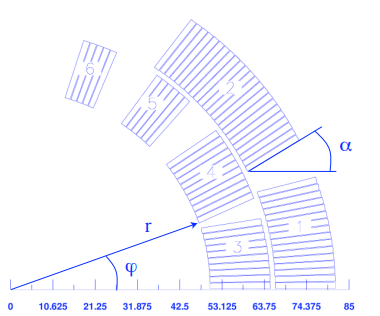
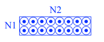
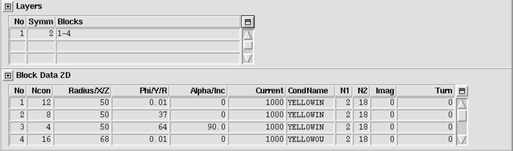
The parameters r (radius), φ (positioning angle) and α (inclination angle) are shown in the Fig. 11.1. The conductor name must be defined in the roxie.cadata-file. The variables N1 and N2 give the discretization in radial and azimuthal direction of the conductors, see Fig. 11.2. This is not equivalent to the number of strands which is given in the input file roxie.data-file under Block Data 2D widget. The three blocks in Fig. 11.3 (left) are defined by the following input table.
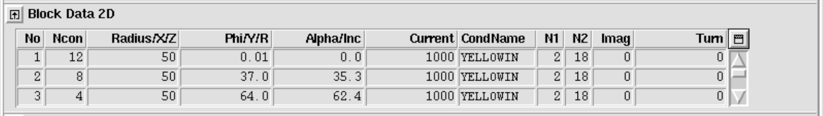
The effect of the turn and image data is illustrated in Fig. 11.3 (right). The input is given below.


The Symmetry option
To make use of symmetries in coil designs the "Symmetric Coil"-option was included in the "Main Options". The cross-section is defined for one pole only and only in the first quadrant. ROXIE does not actually generate the entire coil-geometry - no block- or conductor numbers are given. The "Type of coil/ref. field"-value in the "Global Information"-widget tells ROXIE what kind of magnet symmetry is to be used. The implicitly defined conductors and the sign of the current in each of them are taken into account during field calculation.
At a later stage of development, the layer option was introduced, see Section 11.1.3, which is now standard for many features such as non-linear iron calculations with BEM-FEM coupling or persistent current calculations. The reason for this is that the layer-option generates the entire coil geometry with all conductors. The advantage of the symmetry- over the layer option is that, in order to do a transformation (e.g., during an optimization run) only those blocks (of the first pole) that lie in the first quadrant need to be addressed and all implicitly defined blocks and conductors are transformed accordingly.
With "Dipole" defined in the "Global information"-widget and the "Symmetric coil"-option checked in the "Main Options", the geometry of Fig. 11.3 looks like Fig. 11.4.

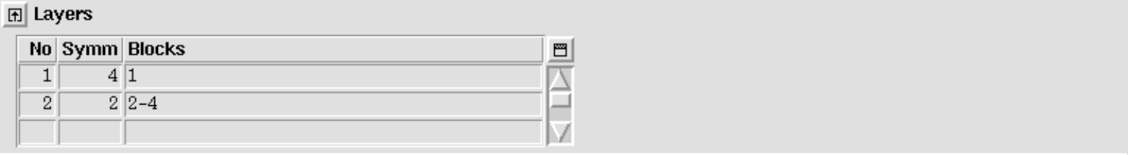
The Layer option
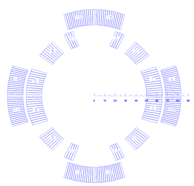
As mentioned above, the layer option, contrary to the symmetry option, generates additional blocks of conductors from the ones that are specified in the "Block Data 2-D"-table. It also allows to assign different geometry types to different layers in the cross-section. To this purpose the "Layer"-widget appears that allows to assign blocks to layers and to specify the respective geometry type. The following input produces the geometry in Fig. 11.5.
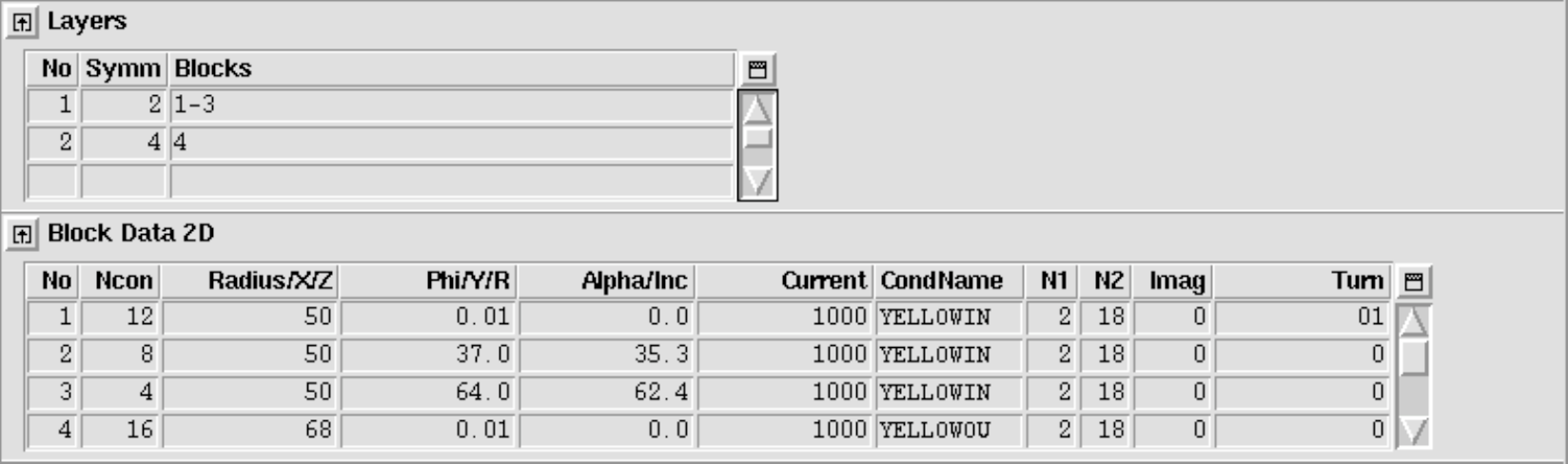
With the layer option switched 'on', the "Type of coil/ref. field"-value in the "Global Information"-widget does not define the coil geometry but only the reference field for harmonic field analysis, see Chapter 6.1. Many transformations in the "Design Variables"-widget apply to individual conductors, blocks or entire layers. A transformation applied to a block in the "Block Data 2-D"-table applies to this block alone and not to the ones generated by the layer option. Therefore it is important to understand the numbering scheme of the generated blocks:\ The first numbers are given to the blocks defined in the "Block Data 2-D"-table. Then the algorithm works layer by layer and block by block, i.e., it will start with block number one in layer one and generate and number the mirrored and turned new blocks before passing on to block 2 in layer 1. Then comes layer 2 and so forth, compare Fig. 11.5. The block numbering can always be checked either in the "Preview Window"-or by printing block numbers in a postscript plots.
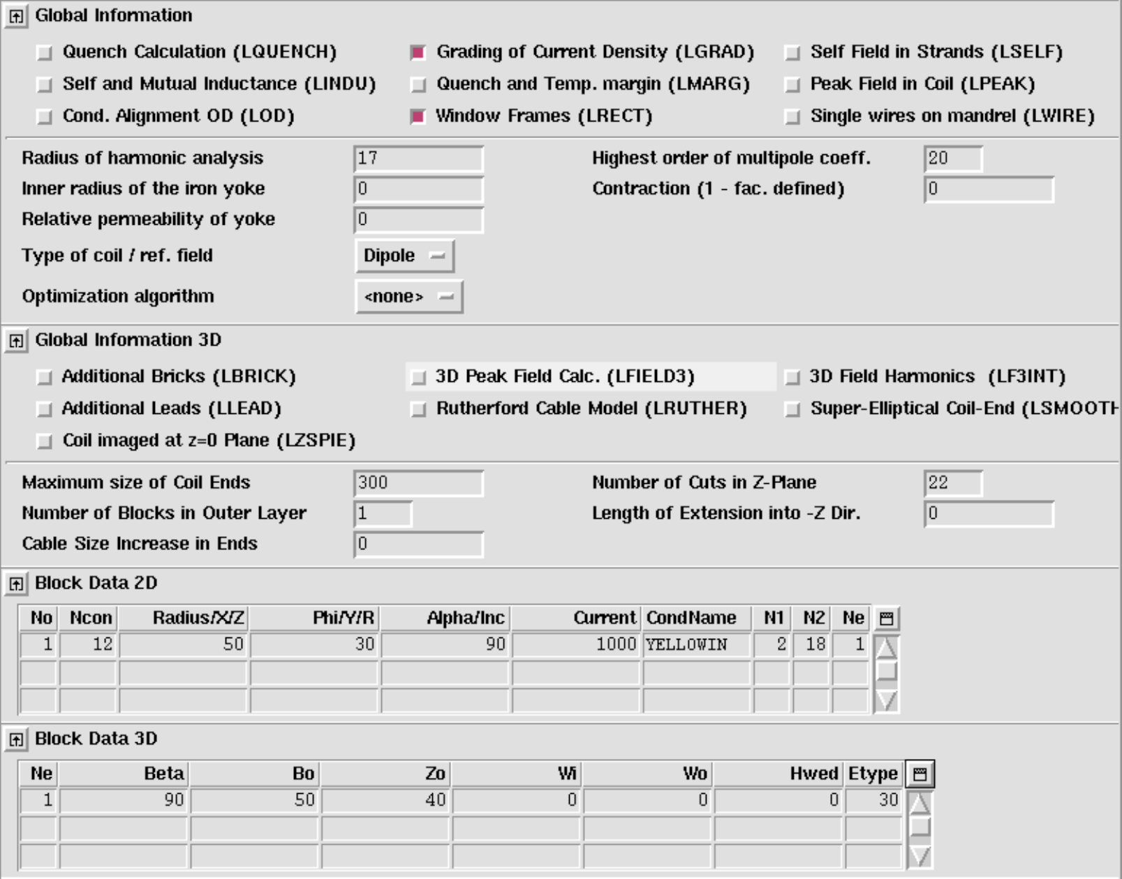
Rectangular cross-section
The standard input option for coil cross-sections is the cosine-theta coil. If other magnet times are to be modeled, this has to be explicitly stated in the input file. The second-most common design variant has rectangular conductor- and block shapes (different window-frame designs, conventional magnets).
The standard option is the "Window Frames"-option in the "Global Variables"-widget. For the input we use same tables and symmetry/layer options as for cosine-theta magnets. Only the meaning of the geometry-data in the "Block Data 2-D"-table changes. The r-variable becomes the x-variable of the block position and the φ- becomes the y-variable. The α-angle is mostly 0 or 90 degrees for window-frame magnets. The following input produces the geometry in Fig. 11.6.
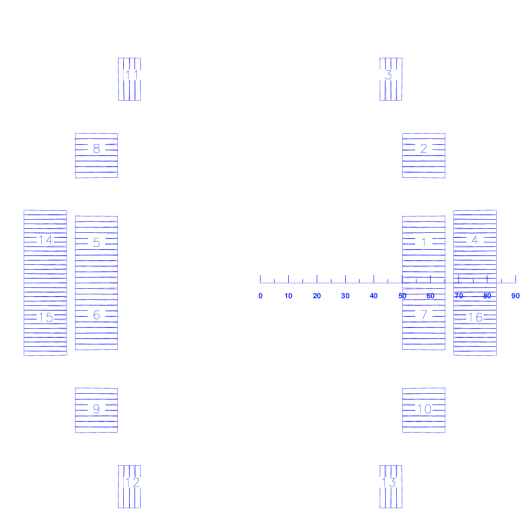
- Note that with the the "Window Frames"-option switched 'on', ROXIE stacks keystoned cables onto each other keeping their mid-planes parallel. The inner width of the conductor defines the conductor spacing. The use of keystoned conductors will thus not make sense, although the program is not going to abort. Keystoned conductors will overlap in a rectangular cross-section.
Elliptical cross-section
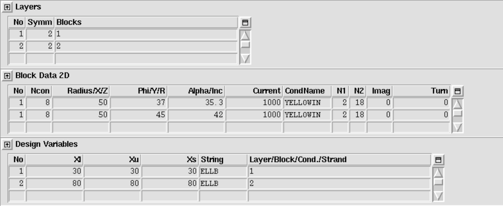
The "ELLB"-option in the "others"-tab of the "Design Variables" allows to allign conductors on an ellipse, rather than a circle. The ellipse uses the radius of the "Block Data 2-D"-table as half-axis along the x-axis and the value specified for "ELLB" for the half-axis along the y-axis. The following input yields the output in Fig. 11.7.

Wires on the mandrel
A third cross-section option is that of individual wires on the mandrel. In that case r- and φ-variables act as in the cosine-theta case, but α becomes the increment angle between individual wires in the block. To use wires on the mandrel the "Single wires on mandrel"-option needs to be clicked. The following input yields the output in Fig. 11.8.

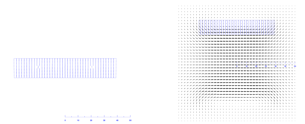
Solenoidal magnets
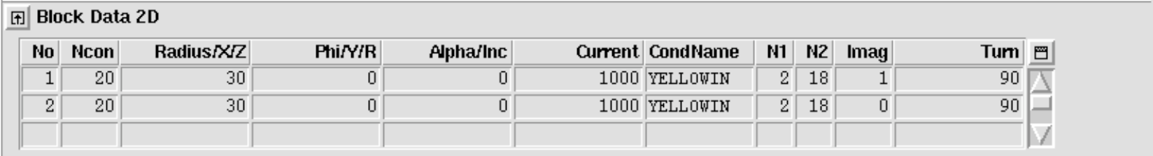
To solve a 2-D solenoidal problem, the Maxwell Equations are solved in cylindrical coordinates. When the "Axi-Symmetry"-option in the "Main Options" is chosen, every wire in the ROXIE model represents a full circular current loop. ROXIE assumes the solenoid axis to lie on the x-axis. Therefore solenoid models are built only in the upper half-plane. The following input (with "Window-Frames"-option clicked) leads to the coil model of Fig. 11.9 (left) and the field shown in 11.9 (right).
Examples of design variable transformations
Coil-blocks (cross-section):
The following input produces the output in Fig. 11.10 (left):
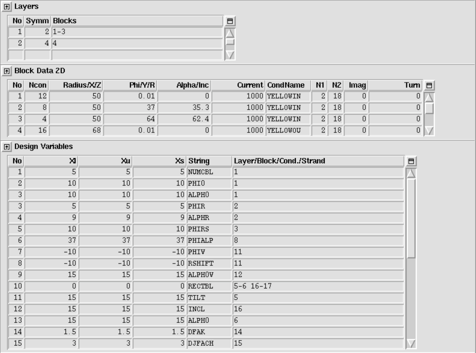
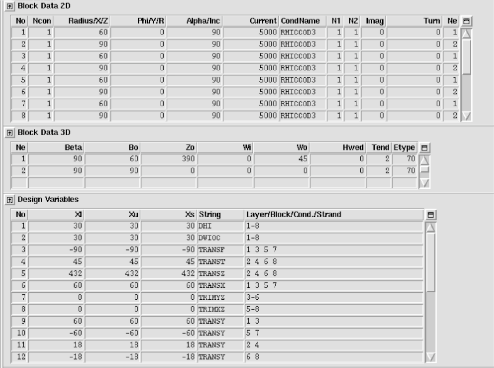
The transformations that have been applied to the design of Fig. 11.5 (all values are either degrees or millimeters or integer numbers) are summarized as follows. Note that the blocks in the fourth quadrant have not been altered and can be used for comparison.
-
The number of conductors in Block 1 was reduced to 5.
-
Block 1 was repositioned at φ1 and α1.
-
Block 2 was positioned relative to Block 1 with φ2 = φ1 + 5 and α2 = α1 +9.
-
Block 3 was positioned at φ3 = φ2 + 10. The angle α3 is chosen such that the resulting wedge between Blocks 2 and 3 is symmetric. (This eliminates a source of error during the coil assembly and helps to reduce costs.)
-
Block 8 was reset to φ8 = α8 = 37.
-
The Block 11 was shifted 10 degrees towards the y-axis and 10 mm towards the center.
-
The inclination angle of block 12 was augmented by 15 degrees.
-
The blocks 5, 6, 16, and 17 were set to be of rectangular shape. Thus the input in the "Block Data 2-D" is read as if the "Window Frames"-option was clicked 'on'.
-
The blocks 5, 6, and 16 are turned in different ways: The "TILT"-option for Block 5 inclines the conductors while leaving the block in upright position; The "INCL"-option for Block 6 leaves the conductors flat but the block is built up in an inclined way; The "ALPH0"-option does the same that a none-zero α angle in the "Block Data 2-D"-table would do: it inclines the entire block and its conductors, the block-shape remaining rectangular.
-
The cable width in Block 14 is increased by a factor of 1.5.
-
The cable height in Block 15 is increased by a factor of 3 - the current in the line currents is increased such that the current density remains unchanged.
Layer:
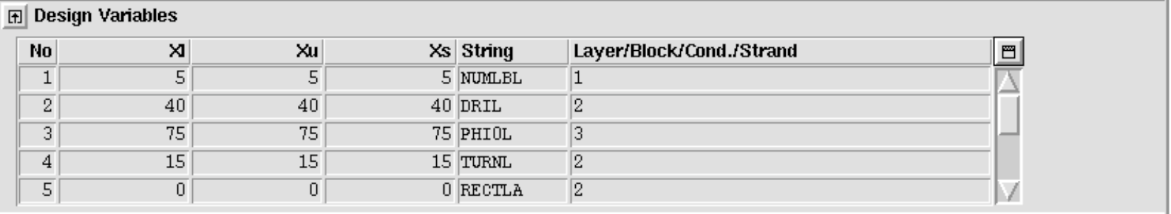
The "Layer"-options in the design variables apply to either an entire layer or to a block in the "Block Data 2-D"-table and all the blocks generated from that one. Several options are used in the following example, compare Fig. 11.10 (right):
-
Block number 1 and hence the Blocks 5, 6, and 7 are assigned five conductors.
-
Block number 2 and hence the Blocks 8, 9, and 10 are set to a mandrel radius of 40 mm.
-
Block 3 and Blocks 11, 12, and 13 are assigned a positioning-angle φ of 75 degrees.
-
Layer 2 is turned by 15 degrees. and all its block are set to be of rectangular type, compare RECTBL-option above.

Conductors:
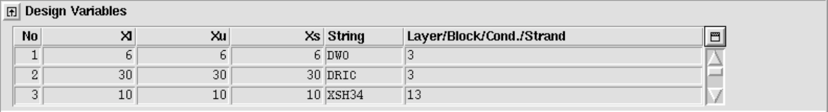
In the "Conductors"-section of the design variables the geometry of conductors can be altered individually or block-wise. The following input yields the coil in Fig. 11.11 (left, the second layer has been omitted).
-
The outer width of the conductors in Block 3 is set to 6 mm.
-
Conductor number 3 is repositioned on a mandrel radius of 30 mm.
-
The outer front of conductor number 13 is shifted in x-direction by 10 mm.
2-D transform (layers and blocks):
In the "2-D Transform (layers and blocks)"-section of the design variables blocks and layers can be shifted and turned. The following input yields the coil in Fig. 11.11 (right).
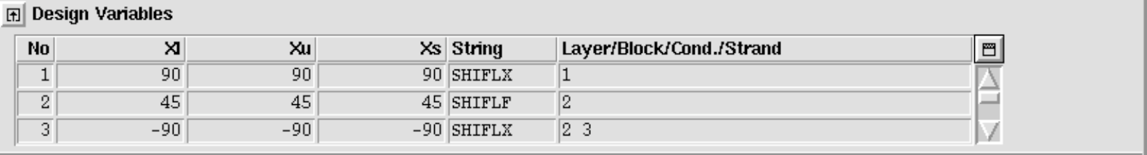
-
Layers 1 and 2 are shifted by 90 mm in opposite x-direction.
-
Layer 2 is turned by 45 degrees. The order is important here
-
Conductor number 3 is repositioned on a mandrel radius of 30 mm.
-
The outer front of conductor number 13 is shifted in x-direction by 10 mm.

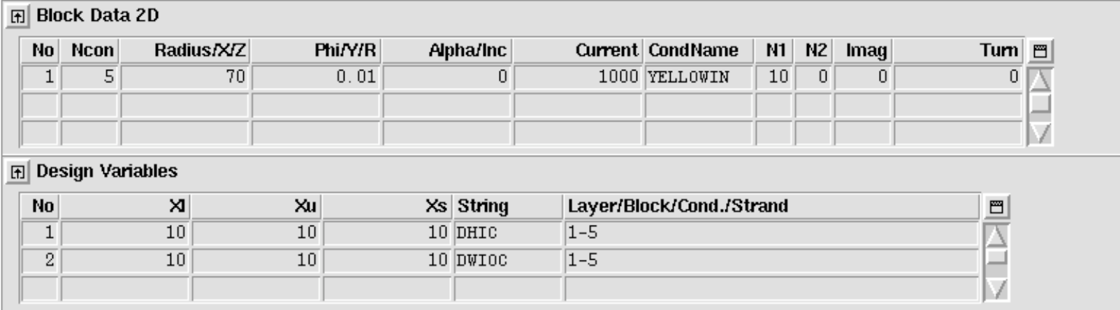
Cable in Conduit
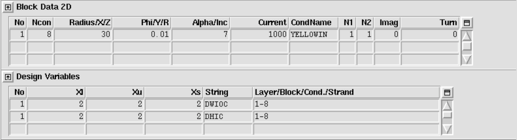
The N1- and N2-parameters in the "Block Data 2-D"-table can be used to define round hollow conductors. To use this feature the N2-parameter is set to 0 while the N1-parameter gives the number of of round conductors to be inscribed into the mantle of the cylinder. This parameter implicitly defines the inner radius of the cylinder. The following input yields the output in Fig. 11.12.

Coil Modeling 3-D
The constant-perimeter coil end
We design a coil end for the cross-section in Fig. 11.5. To this end we switch the "3-D Coil Geometry"-option 'on' in the "Main Options" and enter the following data. The output can be seen in Fig. 11.13 (left).
The coil end in Fig. 11.13](#fig:11_13) is starting point and basically only ensures that the 3-D coil topology is correct. The mechanical quality can be determined from a table given in the .output-file of every 3-D run.
     PERIMETER OF CABLE EDGES (XYZ PLANE, WITHOUT STRAIGHT SECTION) (mm)

            INNER SIDE      OUTER SIDE      CURVATURE (1/MM)   ISOMETRY FACT.
            UPPER LOWER     UPPER LOWER     GEODESIC  NORMAL   MAXIMUM MAXIMUM
     COND.     4     1        3       2                        SQUEEZE STRETCH
        1  230.64  230.67  233.17  233.21 -0.00001    0.00158     0.999  1.141
        2  227.72  227.76  230.24  230.29 -0.00001    0.00160     0.998  1.121
        3  224.79  224.84  227.31  227.37 -0.00001    0.00162     0.997  1.101
        4  221.86  221.92  224.38  224.44 -0.00002    0.00164     0.996  1.082
        5  218.93  219.00  221.44  221.51 -0.00002    0.00165     0.994  1.064
        6  216.00  216.07  218.49  218.57 -0.00002    0.00167     0.993  1.047
      ...     ...     ...     ...     ...      ...        ...       ...    ...
In the case of Fig. 11.13](#fig:11_13) case we find a minimum isometry-value of 0.79. A perfect constant-perimeter end would have 1.0. Optimization of the shape is required (use the BULGE- and CURVAT-options in the "Objectives"-table).
For the plot in Fig. 11.13](#fig:11_13) (right) we use the TRAILZ-option in the "Transform 3-D"-menu of the "Design Variables" and applied it to layer 2, i.e., the inner layer. To set the plot-range right we needed to click the "No shift of Plot Center"-option in the "Plotting Information 3-D"-widget. Note that if you use "Transform 3-D"-options you also have to ensure the correct powering of the transformed blocks or layers. In the case of Fig. 11.13](#fig:11_13) (right) the sign of the currents of blocks 2-4 in the "Block Data 2-D"-table needs to be inversed.
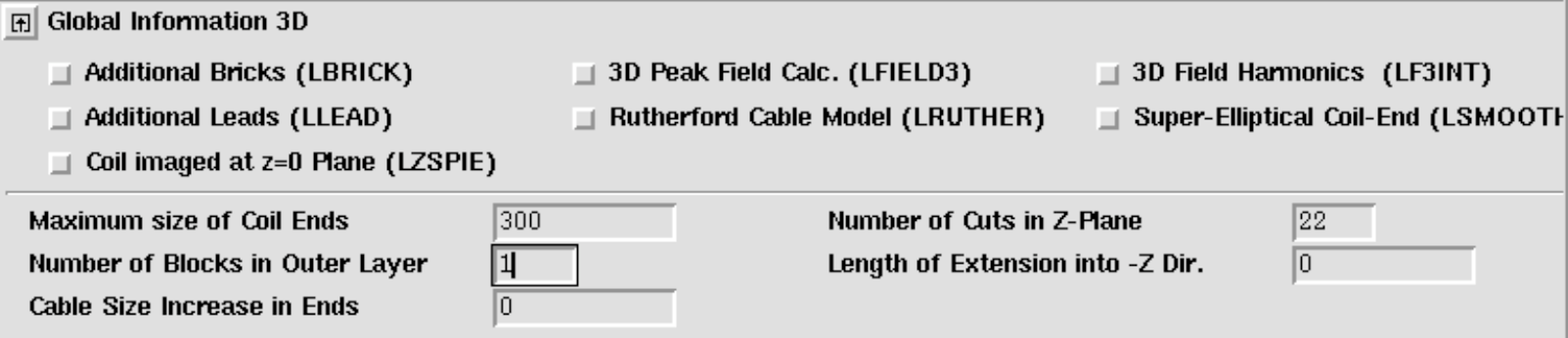
Figure 11.14 shows the effect of the "Super-Elliptical Coil-End"-option in the "Global Information 3-D". The baseline ellipse is replaced by a super-ellips which has a slightly more "rectangular" shape.

Racetrack coil
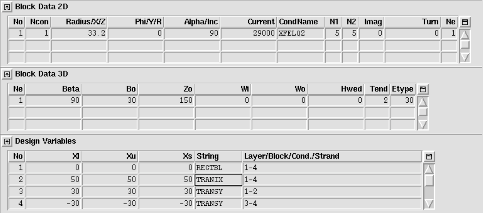
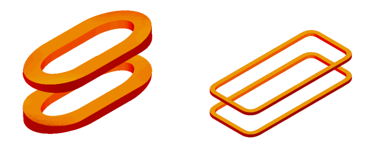
The only coil-end option for Window Frame magnets implemented in ROXIE is the Racetrack Coil. The following input yields the coil end in Fig. 11.15 (left). The "Symmetric Coil"-option from the "Main Options" is selected, as well as the "Plot Imaged at z=0 Plane"-option in the "Plot Information 3-D".
With the following input (option TRANIX) we can introduce a straight part in the racetrack ends, compare Fig. 11.15 (right). The Inserted straight section shifts the straight section apart.
Alternative racetrack coil feature
For lagacy reasons, above method to model racetrack coils uses the same algorithms as the cosine-theta ends. It therefore lacks some flexibility. We propose novel algorithms which reinterprete the "Block Data 3-D"-variables in a way that allows for more flexible racetrack coil-end design.
The new option is selected through the "Etype" (end type) value in the "Block Data 3-D" table. In any case, the "Window Frame"-option in the "Global Information" widget must be switched on.
Soft-way bend racetrack ends
To generate a soft-way (easy-way) bend, the "Alpha"-value of the specific block in the "Block Data 2-D" table must be 90 degrees, the "Beta"-value in "Block Data 3-D" must equally be 90 degrees and the "Etype" value set to 70.
Block data 3-D
| Variable | Description |
|---|---|
| Ne | Row number/number of coil-end definition. |
| Beta | Must be 90 degrees. |
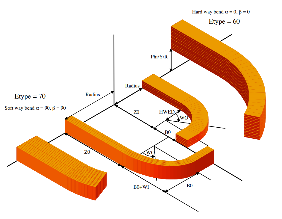
| B0 | Half-axis in x-direction of the ellipse. B0 is measured from the "Radius/X/Z"-variable in the "Block Data 2-D" table towards the origin. |
| Z0 | Straight section in z-direction. |
| Wi | B0 + Wi gives the half-axis in y direction of the ellipse. (Wi = 0 yields a circle.) |
| Wo | Angle in degrees where the coil end stops. Measured from the center of the ellipse. Wo = 0 yields a 90 degree coil end with a straight section towards the (x=0)-plane. |
| Hwed | Not assigned, set to 0. |
| Tend | Not assigned, set to 0. |
| Etype | 70 |
Hard-way bend racetrack ends
To generate a hard-way bend, the "Alpha"-value of the specific block in the "Block Data 2-D" table must be 0 degrees, the "Beta"-value in "Block Data 3-D" must equally be 0 degrees and the "Etype" value set to 60.
Block data 3-D
| Variable | Description |
|---|---|
| Ne | Row number/number of coil-end definition. |
| Beta | Must be 0 degrees. |
| B0 | Half-axis in y-direction of the ellipse. |
| Z0 | Straight section in z-direction. |
| Wi | Not assigned, set to 0. |
| Wo | Angle in degrees where the coil end stops. Measured from the center of the ellipse. Wo = 0 yields a 90 degree coil end with a straight section towards the (x=0)-plane. |
| Hwed | Hwed gives the half-axis in x-direction of the ellipse. It is measured from the "Radius/X/Z"-variable in the "Block Data 2-D" table towards the origin. |
| Tend | Not assigned, set to 0. |
| Etype | 60 |
Examples
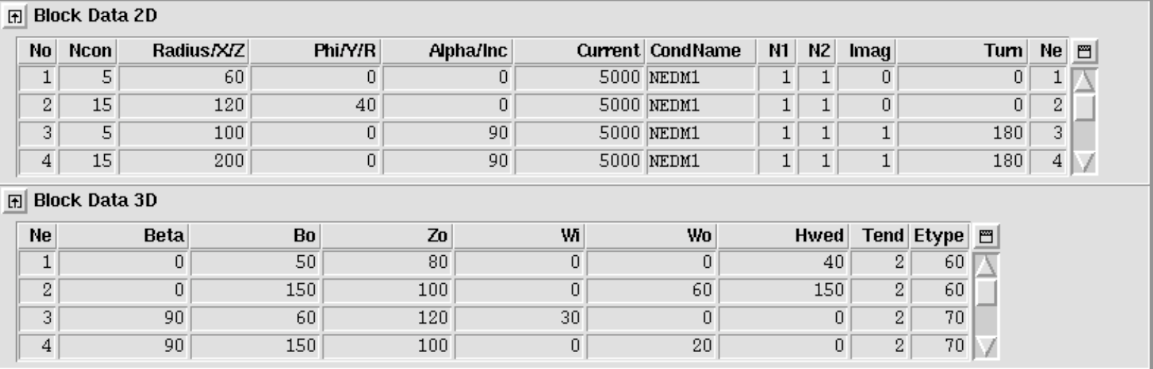
The above-introduced variables are illustrated in Fig. 11.16. The geometry of Fig. 11.16 was generated with the following input
The following input yields the racetrack coil end in Fig. 1.9 (left).
The following input yields the bedstead coil end in Fig. 11.17 (right).

Differential geometry for coil end design
The differential-geometry method for coil-end design yields a more accurate mechanical model of cables in coil ends than the constant-perimeter method. More involved endspacer designs, e.g., for brittle conductors such as Ribbon-type conductors or Rutherford-type cables with a steel core, have a higher chance of success with this method.
Lately we have enabled ROXIE to use coil-end models from the differential-geometry method for field calculation and field-quality optimization. Also the post-processing has been improved. ROXIE can now display differential-geometry coil ends the way it displays constant-perimeter coil ends. 2-D projections of the coils, and endspacer pictures, however, are still bugged.
Differential-geometry coil ends use the same input format in the "Block Data 3-D"-table. All data entered in this table is read and processed in the way it would be for constant-perimeter coil ends. In addition, the user has to specify a number of "Design Variables" from the "Coil Ends (Differential Forms)"-tab. For optimization, the user can choose curvature parameters from the "Coil Ends (Differential Forms)"-tab in the "Objectives"-table. To use differential-geometry coil ends, the "Strips from Darboux Vec."-option in the "Interface options" must be switched on! Otherwise the design-variable input is ignored and a constant-perimeter coil end is produced from the "Block Data 3-D"-table.
The following input generates the output of Fig. 11.18.

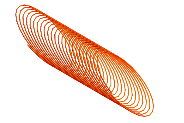
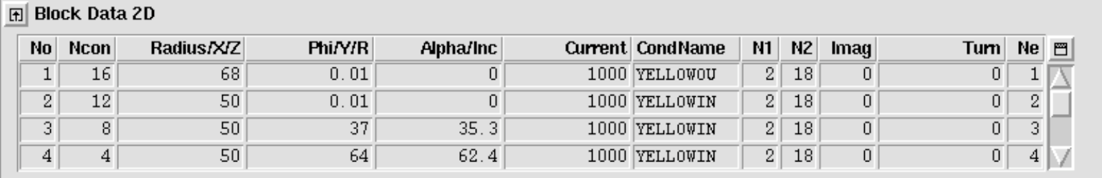
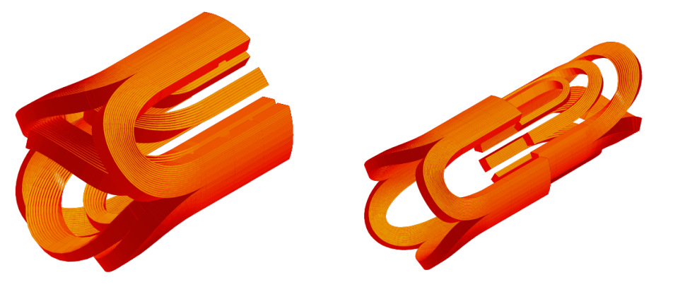
Helical Coils
ROXIE provides a feature to generate helical coils (tilted solenoids, ...). It must be said that helical coils do not quite fit into the program structure of ROXIE which had initially been foreseen for 2-D simulation of cosine-theta magnets. Internally, the helical-coil option creates "additional bricks" (see "Additional Bricks" option). The user might therefore run into a storage-space limitation with the standard ROXIE executable. If this is the case, please contact us and we can compile a version with increased "additonal-bricks capability".
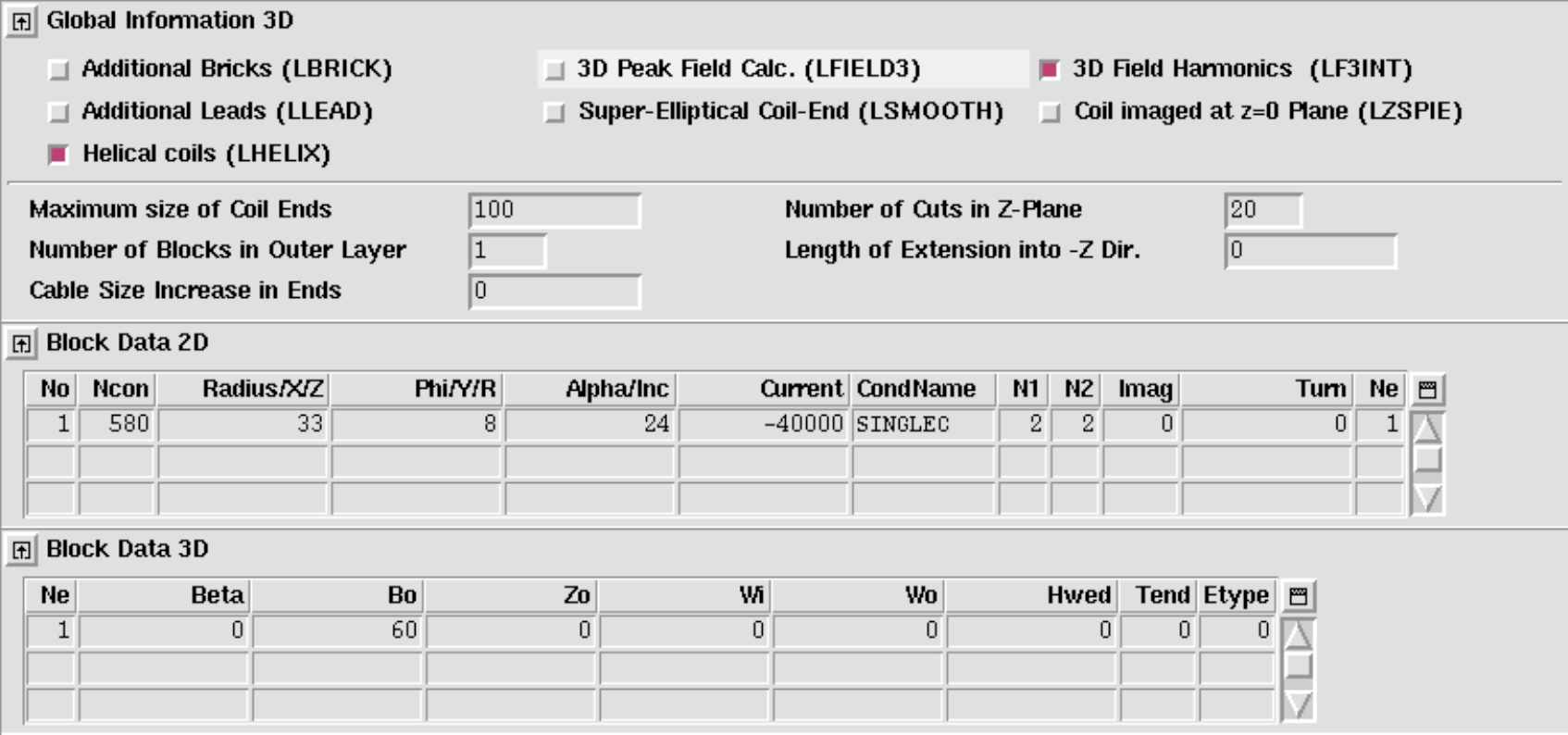
The data in the "Block Data 2-D" and "Block Data 3-D" widget is assigned a different meaning when the "Helical Coil"-option in the "Global Information 3-D" is switched 'on'.
Block data 2-D
| Variable | Description |
|---|---|
| No | Coil number. |
| Ncon | Number of cutplanes. |
| Radius/X/Z | Radius in mm. |
| Phi/Y/R | Pitch in mm. |
| Alpha/Inc | Number of pitches. |
| Current | Conductor current. |
| CondName | Conductor Name. |
| N1 | Radial discretization of conductor. |
| N2 | Azimuthal discretization of conductor. |
| Imag | 0: left-handed screw; 1: right-handed screw. |
| Turn | Starting angle (grad). |
| Ne | Number of coil-end definition that applies to this coil. |
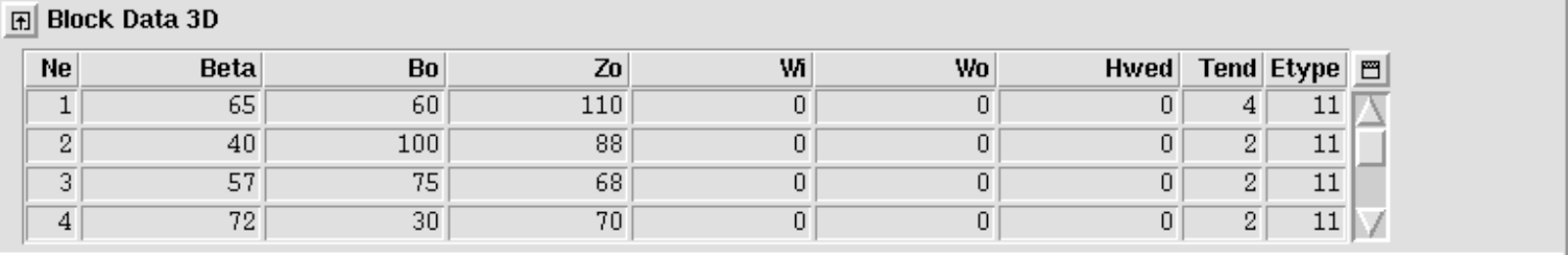
Block data 3-D
| Variable | Description |
|---|---|
| Ne | Row number/number of coil-end definition. |
| Beta | Swing angle; Inclination of helix around y-axis. |
| B0 | Tilt angle; Inclination of helix around x-axis. |
| Z0 | Factor for ellipse half-axis: r_x = r_y (1+Z_0), wind helix on elliptical mandrel. |
| Wi | x-shift. |
| Wo | y-shift. |
| Hwed | z-shift. |
| Tend | Not assigned, set to 0. |
| Etype | Not assigned, set to 0. |
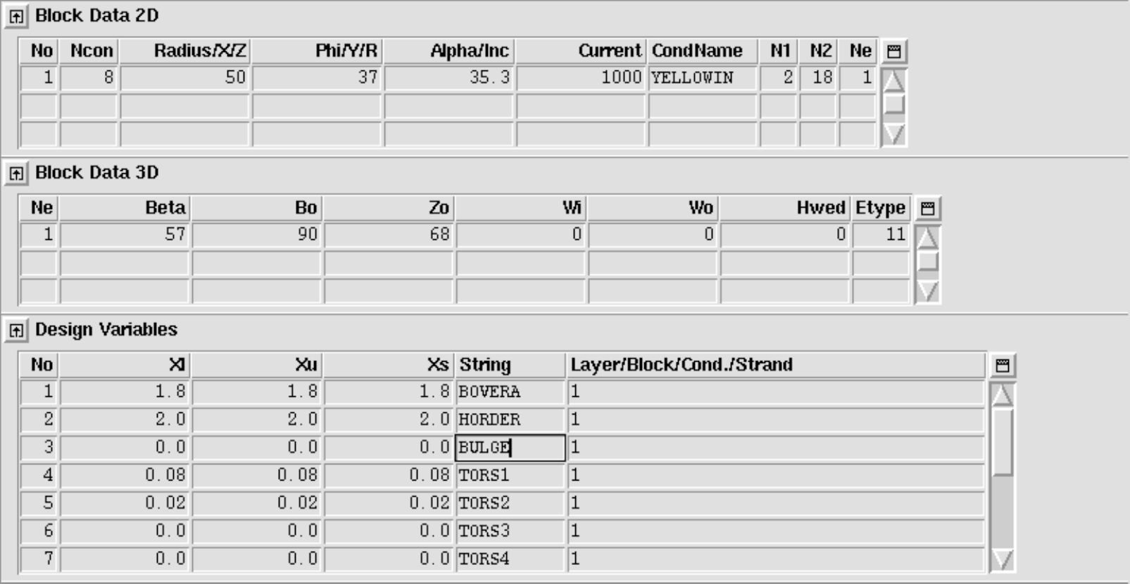
The following input yields the geometry in Fig. 11.19.