Numerical Field Calculation
This chapter treats the calculation of electromagnetic fields in presence of non-linear magnetic material. In 2-D there are two different methods available: A reduced vector-potential formulation for a Finite Element (FEM) approach and a total vector-potential formulation for a hybrid method of boundary elements (BEM) and finite elements. Permanent magnets, non-linear (differential) inductivity, and force calculations are implemented in the BEM-FEM code. In 3-D, ROXIE offers a magnetic scalar-potential- and a magnetic vector-potential formulation for a BEM-FEM calculation. A mesh generator is available for parametric 2-D mesh generation and extrusion of 2-D meshes in z-direction.
The BHDATA file
The roxie.bhdata-file has information on the magnetization curves of
ten different materials, BHiron1 - BHiron10. Each material has one
data block in the roxie.bhdata-file. A block starts with two data
lines which are followed by a data table. The first line gives the
material name BHironX The second line is structured as follows:
| Variable | Type | Description |
|---|---|---|
| num | Integer | Number of measurement points in the table. |
| fil | Double | Stacking factor of the yoke in z-direction. |
| con | Double | Conductivity of the material. |
The tabular data has num lines with entries for B [T] and H
[A/m]:
| Variable | Type | Description |
|---|---|---|
| B | Double | Magnetic induction in Tesla. |
| H | Double | Magnetic field in Ampère/meter. |
Material names and comments are often written following the last data line in a table.
-
Each table in the roxie.bhdata-file must start with the origin, i.e., B=0, H=0.
-
Especially in dense 3-D calculations, the quality of the B(H)-curve determines the speed of convergence. Even non-convergence has been observed, leading to inaccurate results. In cases of non-convergence: check your ROXIE model for input errors; check your B(H)-curve for unphysical behavior; make the mesh coarser.
-
ROXIE assumes that a material is completely saturated if a magnetic induction B exceeds the data given in the roxie.bhdata-file. Above the B-values in the respective data-table ROXIE calculates with the magnetic permeability of free space. This can be a nasty pitfall when you calculate with B(H)-curves of linearly permeable material. Recall, however, that no material retains a high permeability up to very large magnetic induction!
Never forget that a simulation including non-linear material can only be as accurate as the user supplied material-data.
General options for numerical field calculation
FEM/BEMFEM Options
| Option | Description |
|---|---|
| Mesh-Generator | Produce a Finite Element mesh from an .iron-file. |
| Post-proc. only | For non-transient BEMFEM calculations in 2-D only. Such changes to post-processing parameters may be made which do not require recalculation of the problem. |
Global information
Set the "Optimization Algorithm"-variable to "Mutual Inductances in Nl. Circuits" to calculate the differential mutual inductances.
Design variables
Plotting:
| Variable | Description |
|---|---|
| HMOMM | Dimensions in .hmo file given in mm. |
-
The .hmo-file has geometrical data usually given in meters. If, however, the data is to be read in millimeters, the HMOMM-option passes this information to ROXIE.
-
The boundary conditions settings in the "FEM"-, "BEMFEM 2D"-, "BEMFEM 3D (Half)"-, and "BEMFEM 3D (Full)"-menus of the "Design Variables" apply to all 2-D (and 3-D) calculations. Parallel arrows to the symmetry planes correspond to a Dirichlet boundary condition, Bn = 0. Perpendicular arrows correspond to a Neumann boundary condition, Ht.
Objectives
The following options are available for both 2-D algorithms, FEM and BEM-FEM:
Normal Multipoles:
| Variable | Description |
|---|---|
| BIR | Geometry and iron. |
| BIRR | Relative BIR. |
Skew Multipoles:
| Variable | Description |
|---|---|
| AIR | Gemetry and iron. |
| AIRR | Relative AIR. |
Global Values:
| Variable | Description |
|---|---|
| SINDU | Self inductance, see also SectionTransfer function and Section Differential inductance. |
| SINDUD | Differential self inductance, see also Section SectionTransfer function and Section Differential inductance. |
Plotting Information 2-D
Aperture:
| Variable | Description |
|---|---|
| MATR | Field vectors in cross-section. Modulus represented by arrow size. |
| MATRC | Field vectors in cross-section Modulus represented by color code. |
| MATRP | Like MATR but only field from SC-magnetization (PCs, ISCCs analytic model, IFCCs). |
Note that the MATR, MATRC- and MATRP-options have to be used with the "Field-Vector Matrix"-option from the "Interface Options". The option lets the user define the matrix spacing and produces an output file. The reduced field from numerical field calculations is only taken into account if the "Field-Vector Matrix"-option is used.
Coil fields
| Variable | Description |
|---|---|
| ARED | Reduced A. |
| BR | Reduced |B|. |
| BREDX | Reduced Bx. |
| BREDY | Reduced By. |
Interface options
| Option | Description |
|---|---|
| Field-Vector Matrix (Map) | Define a field-vector matrix and produce a file. A widget opens in the GUI. The reduced field from numerical field calculations is taken into account. |
2-D reduced FEM
FEM/BEMFEM Options
| Option | Description |
|---|---|
| Reduced Ar FEM | Use the 2-D reduced vector-potential solver. |
- To use the reduced vector-potential solver, the entire problem domain needs to be meshed. The coils themselves yield a source vector-potential contribution to the solution calculated by Biot-Savart's law. The coil domain thus does not to be modeled in the mesh geometrically, although it needs to be covered by the mesh.
Design variables
FEM:
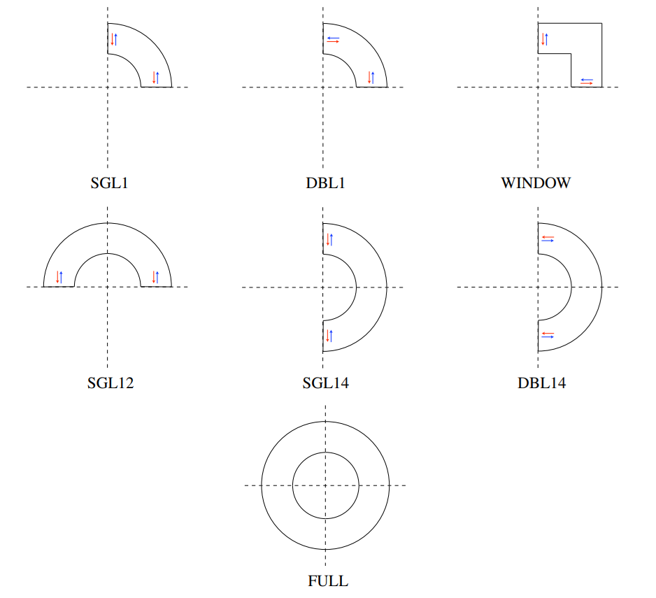
Compare the drawings on page .
| Variable | Description |
|---|---|
| SYMMR | Maximum angle for harmonic analysis within FEM area (90/180/360). Contrary to BEM-FEM calculations a harmonic analysis outside the FEM-domain is not possible! |
| RIHARM | Rescaling of radius for harmonic analysis. The field harmonics are rescaled from the radius value given in the "Global Information" to this radius. A larger value in the "Global Information" might yield better accuracy, depending on the FEM mesh. |
| SGL1 | Single aperture dipole with yoke defined in 1st quadrant. |
| DBL1 | Double apperture dipole / single aperture quadrupole with yoke in 1st quadrant. |
| WINDOW | Window frame dipole with yoke in 1 quadrant. |
| SGL12 | Single/double aperture dipole with yoke in 1st and 2nd quadrant. |
| SGL14 | Single aperture dipole / single aperture quadrupole with yoke in 1st and 4th quadrant. |
| DBL14 | Double aperture dipole with yoke defined in 1st and 4th quadrant. |
| FULL | No symmetry planes. |
Plotting information 2-D
FEM:
| Variable | Description |
|---|---|
| MESH | Finite-elemet mesh. |
| IRON | Iron yoke. |
| AR | Reduced vector potential A. |
| |BRED| | Reduced magnetic field |Br| (iron magnetization only). |
| |BTOT| | Total magnetic field |Bt| (iron and coil). |
| |BS| | Source field |Bs| (coil only). |
| MUE | Relative magnetic permeability μr in iron yoke. |
| MUEFAC | (μr-1) / (μr + 1) in iron yoke. |
2-D BEM-FEM coupling
FEM/BEMFEM Options
| Option | Description |
|---|---|
| Vect.Pot. BEMFEM | Use the 2-D coupling method of Finite Elements (yoke iron) and Boundary elements (coils, air region). |
- Contrary to the reduced vector-potential FEM, with BEM-FEM coupling the air- and coil regions need not be meshed.
Post-proc. only allows to re-process 2-D field plots without running the solver again. Notice that the evaluated field points must not be altered.
Pre-proc and plotting allows to display 2-D and 3-D coils and finite element meshes without running the solver. Notice that the LBEMFEM or the LEDYSON options nevertheless have to be set on true. This has to be done in order to activate the appropriate pre-processors and data transfer routines.
Design variables
BEMFEM 2-D:
Compare the drawings on page .
| Variable | Description |
|---|---|
| SGL1 | Bn(x=0)=0,\;Ht(y=0)=0 (single aperture dipole with yoke defined in 1st quadrant). |
| DBL1 | Ht(x=0)=0,\;Ht(y=0)=0 (double aperture dipole / single aperture quadrupole with yoke in 1st quadrant). |
| WINDOW | Bn(x=0)=0,\;Bn(y=0)=0 (window frame dipole with yoke in 1st quadrant). |
| SGL12 | No boundary condition at x=0, Ht(y=0)=0 (single/ double aperture dipole with yoke in 1st and 2nd quadrant). |
| SGL14 | Bn(x=0)=0, no boundary condition at (y=0) (single aperture dipole / single aperture quadrupole with yoke in 1st and 4th quadrant). |
| DBL14 | Ht(x=0)=0, no boundary condition at (y=0) (double aperture dipole with yoke defined in 1st and 4th quadrant). |
| FULL | No symmetry planes. |
| CURRY | Index to coil (FEM coils). Not yet documented. |
| FRINGR | Radius of fringe field calculation |
| FRINGA | Maximum angle for fringe field calculation (from x-axis). |
| ACCIMP | Improved accuracy of the GMRES iteration of BEMFEM (70dB instead of 55dB). |
| NSTEPS | Set maximum number of steps in Newton-Algorithm to 10 (instead of 50). |
- The FRINGR- and FRINGA-options produce plots in the .post-files that show the magnetic field (components and total) on an arc around the coordinate centre.
Plotting information 2-D
BEMFEM:
| Variable | Description |
|---|---|
| MESH | Finite-element mesh. |
| IRON | Iron yoke. |
| AR | Total vector potential A in FEM domain. |
| |BTOT| | Total magnetic field |B| in FEM domain. |
| MUE | Relative magnetic permeability μr in iron yoke. |
| MUEFAC | (μr-1) / (μr + 1) in iron yoke. |
- To plot the iron yoke and/or information on the iron yoke, the IRON-option must be specified together with the field, e.g., 'IRON AR' will plot the vector potential in the yoke, whereas only 'AR' will not have any effect.
3-D BEM-FEM coupling
With the "3-D Coil Geometry"-option 'on' in the "Main options", ROXIE expects also a 3-D mesh and uses 3-D numerical algorithms. The choice in the algorithms is between a total vector-potential BEM-FEM formulation and a total scalar-potential BEM-FEM formulation. All options (other than the choice of a formulation) in this section apply to both, the vector-potential- and the scalar-potential formulation.
FEM/BEMFEM Options
| Option | Description |
|---|---|
| Vect.Pot. BEMFEM | 3-D coupling method of Finite Elements (yoke iron) and Boundary elements (coils, air region). The problem is formulated in terms of the 3 components of the magnetic vector potential. |
| PSItot BEMFEM | 3-D coupling method of Finite Elements (yoke iron) and Boundary elements (coils, air region). The problem is formulated in terms of the magnetic scalar potential. |
- The "Vect.Pot. BEMFEM"-option, due to the linear, mesh-point-wise approximation of the three components of the magnetic vector potential, cannot approximate jumps in the vector potential. These jumps occur on sharp edges and corners in the presence of important jumps of the magnetic permeability at the edge/corner. These problem-types might lead to unphysical and inaccurate results.
The "PSItot BEMFEM"-option avoids the above problem. It is available, however, only for single-aperture magnets, i.e., if the coil is centered at the origin.
Design variables
BEMFEM 3-D (half):
The "half"-versions of boundary conditions assume that the iron yoke is mirror-symmetric with respect to the (z=0)-plane. Compare the drawings on page .
| Variable | Description |
|---|---|
| SGLH1 | Bn(x=0)=0,\;Ht(y=0)=0 (single aperture dipole with yoke defined in 1st quadrant). |
| DBLH1 | Ht(x=0)=0,\;Ht(y=0)=0 (double aperture dipole / single aperture quadrupole with yoke in 1st quadrant). |
| WINDOH | Bn(x=0)=0,\;Bn(y=0)=0 (window frame dipole with yoke in 1st quadrant). |
| SGLH12 | No boundary condition at x=0, Ht(y=0)=0 (single- / double aperture dipole with yoke in 1st and 2nd quadrant). |
| SGLH14 | Bn(x=0)=0, no boundary condition at (y=0) (single aperture dipole / single aperture quadrupole with yoke in 1st and 4th quadrant). |
| DBLH14 | Ht(x=0)=0, no boundary condition at (y=0) (double aperture dipole with yoke defined in 1st and 4th quadrant). |
| FULLH | No symmetry planes. |
BEMFEM 3-D (full):
The "full"-versions of boundary conditions assume that the iron yoke has no symmetries in z-direction.
| Variable | Description |
|---|---|
| SGLF1 | Bn(x=0)=0,\;Ht(y=0)=0 (single aperture dipole with yoke defined in 1st quadrant). |
| DBLF1 | Ht(x=0)=0,\;Ht(y=0)=0 (double aperture dipole / single aperture quadrupole with yoke in 1st quadrant). |
| WINDOF | Bn(x=0)=0,\;Bn(y=0)=0 (window frame dipole with yoke in 1st quadrant). |
| SGLF12 | No boundary condition at x=0, Ht(y=0)=0 (single- / double aperture dipole with yoke in 1st and 2nd quadrant). |
| SGLF14 | Bn(x=0)=0, no boundary condition at (y=0) (single aperture dipole / single aperture quadrupole with yoke in 1st and 4th quadrant). |
| DBLF14 | Ht(x=0)=0, no boundary condition at (y=0) (double aperture dipole with yoke defined in 1st and 4th quadrant). |
| FULLF | No symmetry planes. |
Objectives
Peak Fields:
| Variable | Description |
|---|---|
| STRFEL | Field along strand (with LEND and line-field option). |
Peak field calculations in 3-D with iron are computationally extremely costly and therefore not implemented in ROXIE. The 'STRFEL' option allows to calculate the field along a single strand in 3-D, including source- and iron field. To use 'STRFEL' you have to specify the strand number in the "Nor" column, "PLOT" in the "Oper" column and 1 and 1 for the remaining columns. Furthermore you have to switch "on" the "Field along a Line (2-D,3-D)" option in the "Interface Options" and supply dummy values. ROXIE then uses its algorithms for a field along a line. The points along the line are located in the line-current segments which constitute a strand. For an example see Section 3D Peak Field Calculation.
Plotting information 3-D
In 3-D plots, the iron yoke is always represented when the respective "FEM/BEMFEM Options"-options are 'on'. Unless the 'SUN'-option is chosen, the magnetic induction is displayed on the surface elements of the iron yoke.
Transfer functions
Main options
| Option | Description |
|---|---|
| Transfer Function | Calculate field at different levels of excitation. |
- The "Transfer Function"-option triggers a series of successive calculations. It is not a time-stepping. No time-transient effects are taken into account. The "Transfer Function"-option is primarily used to determine the influence of yoke saturation on the field quality.
Objectives
Global values:
| Variable | Description |
|---|---|
| NIB | N I / Bref |
| BOVERI | Transfer function Bref/I (in T/kA). |
| SINDU | Self inductance, see Section Differential Inductance. |
| SINDUD | Differential self inductance, see also Section Differential Inductance. |
- With the "Self and Mutual Inductance"-option switched 'on' in the "Global Information", the SINDU- and SINDUD-options let you evaluate the linear and differential inductance of the magnetic circuit during a transfer function. A plot is produced if the "Postscript Plots"-option is 'on' that shows L and L_\mathrm{d} as a function of excitation.
Normal multipoles (vers. excit.):
| Variable | Description |
|---|---|
| BIRI | Normal multipoles (injection field level). |
| BIRRI | Relative BIRI. |
| BIRN | Normal multipoles (nominal field level). |
| BIRRN | Relative BIRN. |
| BIRD | Normal multipoles (variation). |
| BIRRD | Relative BIRD. |
Skew multipoles (vers. excit.):
| Variable | Description |
|---|---|
| AIRI | Skew multipoles (injection field level). |
| AIRRI | Relative AIRI. |
| AIRN | Skew multipoles (nominal field level). |
| AIRRN | Relative AIRN. |
| AIRD | Skew multipoles (variation). |
| AIRRD | Relative AIRD. |
-
For the BIRI- and AIRI-options the injection field level is assumed to be the first level in the "Transfer Function"-widget.
-
For the BIRN- and AIRN-options the nominal field level is assumed to be the last level in the "Transfer Function"-widget.
Transfer function
The input in the line of the "Transfer Function"-widget is a space-delimitted enumeration of excitation factors. The currents given in the "Block Data 2-D"-widget are scaled by each of the given values successively.
Permanent magnets in 2-D
FEM/BEMFEM options
| Option | Description |
|---|---|
| Permanent Magnets | Read in magnetization data from .VEFI-file and assign to areas in .iron-file according to design variables (see below). |
Design variables
BEMFEM 2-D:
| Variable | Description |
|---|---|
| HARD | Index to magnetization vector field compare Section Permanent magnets in 2d. |
- For the HARD-option, the value in the "Xl, Xu, Xs"-columns of the table is of integer type. It points to a vector field defined in the so-called .VEFI-file, see SectionVefi file. The number in the right column of the design variables points to an area in the .iron-file. In fact, it rather points to a material name. A number 2 in the right table corresponds to the second material name in the first block of the .hmo-file, see Section HMO file. You therefore need to check the .hmo-file in a first run before you can assign vector fields. The magnetic characteristic of the permanent magnet is given in the roxie.bhdata-file under the respective material name. For an example see Section Permanent magnets in 2d.
The VEFI file
The .VEFI-file defines vector fields for the calculation of (hard) permanent magnets in 2-D. The .VEFI-file is used in connection with an .iron-file and a .data-file that uses the option 'HARD' in the "Design variables"-table. For an example see Section Permanent magnets in 2d.The first line of the .VEFI-file has two parameters:
| Variable | Type | Description |
|---|---|---|
| NFIELD | Integer | Number of vector fields to be defined. |
| TBLOCK | Integer | Total number of building blocks. |
Then follows the definition of each vector field that consists of a header record and a sequence of pairs of records specifying the building blocks. The header record has three parameters:
| Variable | Type | Description |
|---|---|---|
| IFIELD | Integer | Consecutive number of vector field. |
| NBLOCK | Integer | Number of building blocks for the vector field. |
| FACT | Double | Scaling factor for the vector field. |
The first line of the building block data yields the following parameters:\
| Variable | Type | Description |
|---|---|---|
| IBLOCK | Integer | Consecutive number of building block. |
| PCOSY | Integer | Pointer to the frame of reference. |
| ITYP | Integer | Type of coordinate system (1: Cartesian, 2: cylindrical). |
| IDIR | INTEGER | Direction of the vector field (+/-1: first, +/-2: second, +-3: third basis vector). |
| ILIMIT(3) | Integer | Flags specifying the type of inequality for the range of each coordinate (see below). |
The second line has the limit parameters:\
| Variable | Type | Description |
|---|---|---|
| XYZLO(3) | Double | Lower limits for the range of each coordinate. |
| XYZHI(3) | Double | Upper limits for the range of each coordinate. |
The ILIMIT flags have the following meaning, e.g. for the x-coordinate:
ILIMIT=0 -∞ ≤ x ≤ ∞
ILIMIT=1 -∞ ≤ x ≤ xhigh
ILIMIT=2 xlow. ≤ x ≤ ∞
ILIMIT=3 xlow. ≤ x ≤ xhigh