SC-Related Time-Transient Effects
This chapter introduces ROXIE features to simulate superconductor magnetization, the persistent currents (PCs), as well as Eddy-Current effects on the strand level, the interfilament coupling currents (IFCCs) and on the conductor level, the interstrand coupling currents (ISCCs) in Rutherford-type cables. The PC models have been developed at CERN whereas the analytical models for IFCCs and ISCCs are based on models by M. Wilson. A network model for more accurate modeling of ISCCs is equally available.
All models in this chapter have in common that they should be used with the "Layer Definition"-option in the "Main Options". For the use of semi-analytical models, the "Symmetry: 0: Gen., 1: in1, 2: 2in1"-option in the "Time Transient Effects"-widges allows to make use of coil symmetries nevertheless.
The term 'SC magnetization' is used for all quantities in ROXIE's semi-analytical models, also for Eddy-Current effects such as IFCCs and ISCCs. These effects are modeled as magnetizations on the strand/cable level.
Semi-analytical models for SC magnetization
The main material parameters for the SC magnetization models are found in the roxie.cadata-file which is editable via the "Open cable data window (.cadata)"-entry in the "Run"-menu. Main input parameters are found in the "Time Transient Effects"-widget.
The analytical formula to compute the strand-magnetization from PCs is given by:
The IFCCs are evaluated from:
The user is required to provide the wire filling-factor λw, the wire twist-pitch lw and the effective resistivity ρeff which consists of a constant part ρ0 and a coefficient due to magneto resistance ρ1.
ISCCs are calculated as the sum of the following components:
The user provides the cable twist-pitch lc, the contact- and adjacent resistances, Rc, Ra and the cable dimensions b (narrow side - the mean value is taken for keystoned cables) and c (broad side).
Main options
| Option | Description |
|---|---|
| Time Transient | Perform a time-stepping, evaluate superconductor magnetization. |
Design variables
Layers:
| Variable | Description |
|---|---|
| FILDIL | Filament Diameter in layer (in \mum). |
Coil Blocks (Cross-Section):
| Variable | Description |
|---|---|
| FILDIA | Filament Diameter in block (in \mum). |
| TEMPBL | Operation temperature in block. |
- The TEMPBL-option sets the operation temperature in specified blocks, e.g., to test the impact of an inhomogeneous cooling on the margins to quench or on persistent currents. The TEMPBL-option is used with features that use the critical-current fit function and not with those that use the linear approximation thereof.
Magnetization:
| Variable | Description |
|---|---|
| STRPRI | Print info of specified strand(s). |
| ABSCIS | Field harmonic versus excitation- (B_n versus I) plot (see objectives): take I of specified block number (default is block 1). |
Objectives
Magnetization data:
| Variable | Description |
|---|---|
| MSTR | Magnetization in filament. |
| BSTR | Magnetic induction in filament. |
| MSTRT | Magnetization modulus. |
| BSTRT | Magnetic modulus. |
| MSTRF | Angle of magnetization. |
| BSTRF | Angle of magnetic induction. |
| AB | Skew and normal harmonics in one plot. Currently not supported. |
| DTRF | Current factor of block as function of time. |
- The MSTR*- and BSTR*- and DTRF-options plot excitation, field and resulting strand magnetization. The x-axis data varies between the chosen analytical model: IFCCs and PCs-option 1 and 3 yield plots over the excitation current (of the first block); ISCCs and PCs-option 4 plot over the time. For the latter two options, the MSTRF- and BSTRF-options yield the angular information of the respective strand's magnetization and excitation.
Plotting Information 2-D
Coil fields:
| Variable | Description |
|---|---|
| MX | SC magnetization (x-component). |
| MY | SC magnetization (y-component). |
| |M| | SC magnetization (modulus*sign). |
| MMOD | SC magnetization (modulus). |
| M | SC magnetization vectors. |
| P | Losses per strand in W/m. The losses due to filament/strand/cable-magnetization is computed as \frac{\mathrm{d}\mathbf{M}\cdot \mathbf{B}}{\mathrm{d}t}. For the ISCC magnetization model this yields the Ohm's losses. |
| PINT | The integral \int \mathbf{M}\cdot\mathrm{d}\mathbf{B} is calculated and updated at every time step. The result is the integrated magnetization losses for PCs, IFCCs and the ISCC magnetization model in J/m. |
| BPERP | B perpendicular to broad face of the conductor. |
| BPARA | B parallel to broad face of the conductor. |
Bn strand contr. of M:
| Variable | Description |
|---|---|
| M1 | B_1 contribution of SC magnetization. |
| M2 | B_2 contribution of SC magnetization. |
| M3 | B_3 contribution of SC magnetization. |
| M4 | B_4 contribution of SC magnetization. |
| M5 | B_5 contribution of SC magnetization. |
| M6 | B_6 contribution of SC magnetization. |
| M7 | B_7 contribution of SC magnetization. |
| M8 | B_8 contribution of SC magnetization. |
| M9 | B_9 contribution of SC magnetization. |
| M10 | B_{10} contribution of SC magnetization. |
| M11 | B_{11} contribution of SC magnetization. |
Time Transient Effects
Options
| Option | Description |
|---|---|
| IFCC (Wilson) | Interfilament Coupling Currents - analytical model by M. Wilson. |
| ISCC (Wilson Analytic) | Interstrand Coupling Currents - analytical model by M. Wilson. |
| Nonlinear Inner Iterations | Only with BEMFEM calculations of a nonlinear iron yoke are 'on'. This option makes ROXIE recalculate the contribution of the iron yoke at every step of the inner magnetization iteration. If 'off' the nonlinear iron yoke is only calculated before the first and after the last step of the inner iteration. |
| Plotting Magn. Fields Only | The harmonic analysis is done only from the fields due to SC magnetization. The perturbation of the field quality due to SC magnetization is calculated. |
-
The "IFCC (Wilson)"-option uses a formula to evaluate the total strand magnetization which does not take into account those Eddy-Current loops that close in the outer copper coating of the strand, i.e., it assumes a highly resistive barrier between the filaments and the outer coating.
-
The "ISCC (Wilson Analytic)"-option a homogeneous magnetization in each conductor. The nature of ISCCs is better represented in a network model, see Section 9.2{reference-type="ref" reference="sec:transientnetwork"}.
Parameters
| Variable | Description |
|---|---|
| PC: 0:None; 1,3:1D; 4:Vector | Persistent Current (PC) calculations. '0': no PC calculation; '1','3': two implementations of the same 1D persistent current model; '4': vector hysteresis model for field-changes in modulus and direction. |
| Symmetry: 0: Gen., 1: 1in1, 2: 2in1 | To use time-transient effects, you should use the layer-option which generates the full coils. If there is a symmetry, then you may specify only the blocks first quadrant (in the right aperture) in the "Block spec. (Peak fields, Forces, FEM plots)"-widget. SC-magnetization is then only evaluated in these blocks. The contribution of the other blocks in the layer is considered automatically. |
| Start Time for Loss Calculation | Start time for loss calculation (in seconds). |
| End Time for Loss Calculation | End time for loss calculation (in seconds). |
| Start Time for Multipole Variation | The BIRD- and BIRRD-options in the "Objectives"-table calculate the multipole variation during a transfer function or during a transient calculation. For the latter, the time-frame for the variation can be given. |
| Start Time for Multipole Variation | The BIRD- and BIRRD-options in the "Objectives"-table calculate the multipole variation during a transfer function or during a transient calculation. For the latter, the time-frame for the variation can be given. |
| Maximum Number of Iterations | Maxim number of iterations in the determination of the SC magnetization. |
Time-Grid definition
The table for the definition of a stepping time-grid has the following columns.
| Variable | Description |
|---|---|
| No | Number of interval. |
| Ts | Start time of interval (seconds). |
| Te | End time of interval (seconds). |
| Steps | Number of time steps in interval. |
Excitation function definition
The table for the definition of excitation functions for each block of conductors has the following columns. Each block can be assigned a number of successive excitation functions over time intervals that need not be the same as the stepping intervals in the table above. At every step of the stepping table each block must be assigned one (and only one) excitation function.
| Variable | Description |
|---|---|
| No | Number of excitation function definition. |
| Ts | Start of excitation interval. |
| Te | End of excitation interval. |
| Function | Predefined excitation functions. |
| 1: Linear ramp, from A(T_\mathrm{s}) to B(T_\mathrm{e}), | |
| 2: A+B\cos(C t + D), | |
| 3: Parabolic from A(T_\mathrm{s}) to B(T_\mathrm{e}) with acceleration C, \frac{C}{2}t^2 + \beta t + \gamma, where \beta and \gamma are calculated to match A and B at T_\mathrm{s} and T_\mathrm{e}. | |
| 4: Exponential from A(T_\mathrm{s}) with derivative B, | |
| 5: Quadratic from A(T_\mathrm{s}) with maximum slope C and linear slope increase during B\,\Delta T, compare Fig. 9.1. Parameter D is '1': ramp up, '2': ram up and down, '3': ramp down. | |
| A | Function parameter A. |
| B | Function parameter B. |
| C | Function parameter C. |
| D | Function parameter D. |
| Blocks,Layers | With the "Symmetric Coil"-option blocks are assigned the excitation function in the specified time interval. With the "Layer Definition"-option, individual layers are assigned excitation functions. |
- Function number 5 with D=2: In this case the \Delta T in Fig. 9.1{reference-type="ref" reference="fig:gsiexcitationfunction"} is set to (T_\mathrm{e}-T_\mathrm{s})/2.
Network model of Interstrand Coupling Currents
For the simulation of interstrand coupling currents an electrical-network model is implemented in ROXIE. In this model, interstrand coupling currents are not treated as an additional magnetization of the SC conductors (as in the above analytical model) but as additional (positive and negative) line currents in the position of each strand.
The network model of ISCCs cannot be used with nonlinear iron.
Plotting Information 2-D
Current distribution:
| Variable | Description |
|---|---|
| ICC | Interstrand coupling currents. |
Time transient effects
Options:
All analytical SC magnetization models must be 'off'.
| Option | Description |
|---|---|
| ISCC (Network Model) | Network model (without inductance matrix for interstrand coupling current determination. |
| LICC + Mut. Inductances | Compute and use the inductance matrix in the network model. |
| Plotting Magn. Fields Only The harmonic analysis is done only from the fields due to ISCCs. The perturbation of the field quality due to ISCCs is calculated. |
Parameters:
The "Symmetry"-parameter should be set to zero and all blocks be specified in the "Block spec. (Peak fields, Forces, FEM plots)"-widget.
Time-grid definition:
The same time-grid definition is used as for the analytical models.
Excitation Function Definition:
The excitation function is defined in the same way as for the analytical models.
Quench Calculation
ROXIE features a new quench simulation tool. The tool is currently under development. A first version is available in ROXIE 9.3. This version corresponds to the IEEE paper [@Schwerg:2007lr] by Nikolai Schwerg. It is highly recommended to read this paper before using the algorithm.
To do quench simulation, the following options need to be set
-
"Quench Calculation" in "Global Information".
-
"Self and Mutual Inductance" in "Global Information".
-
"Quench and Temperature Margin" in "Global Information".
-
"Peak Field in Coil" in "Global Information".
-
"Time Transients" in "Main Options". For a description of the "Time Transients"-widget in the context of quench, see Section 4.3{reference-type="ref" reference="sec:quench_ex"}.
-
"Layer Definition" in "Main Options".
-
All conductors must be specified in the "Block spec." widget.
-
A winding scheme needs to be specified, see Section 4.3{reference-type="ref" reference="sec:quench_ex"}.
Quench calculation with ROXIE automatically produces a number of files for post-processing with gnuplot:
- The roxie.dat file contains about 30 quantities over time, one row per time-step. The description is found in the last line of the file.
roxie.QUENCH is an event-history of the quench simulator.
-
.xdat-files contain relevant data per conductor and time-step.
-
.xsp-files are overwritten in each time step. By calling
gnuplot load "filename.xsp"
you can plot cross-section data.
- .gnu-files are gnuplot macros to display .xdat and files and the roxie.dat file. They are loaded by
gnuplot load "filename.gnu"
The files can also be viewed during a simulation run. Update a view by typing the gnuplot command "e".
-
Overview.gnu shows the characteristic quantities (voltages, current, resistances, and temperature).
-
Powers.gnu shows the dissipated power over the coil cross-section.
-
Xsections.gnu shows cross-section data (temperature margin, field, resistances, and temperature).
-
Voltages.gnu shows voltages versus time (terminal voltage, induced voltage, ohmic voltage, dump resistor voltage, diode voltage).
The following gnuplot macros produce postscript files
-
Report.gnu reports the most characteristic quanities over time and in the cross-section.
-
roxie.dat.gnu Illustrates the roxie.dat file (see above).
Note that all the output files can take several hundreds of megabytes of disc space!
Global information
| Option | Description |
|---|---|
| Quench Calculation | Perform a quench simulation. |
| Winding Scheme Input | Change the conductor numbering in the preview window according to winding scheme. |
-
For the quench algorithm the user is required to supply the winding scheme of the magnet's coils. The "Winding Scheme Input"-option serves to debug the winding-scheme input.
-
The winding-scheme input is documented in an example in Section 4.3{reference-type="ref" reference="sec:quench_ex"}.
Design variables
Quench, Inductance:
| Variable | Description |
|---|---|
| QUENCH | Conductor number in which quench originates. Use the conductor number from the preview window with the "Winding Scheme Input"-option 'off'. |
| QLOSST | Time constant of interstrand coupling currents. |
| HEATTT | Heat transfer coefficient from turn to turn per unit length. |
| HEATER | Heater delay (in seconds) for specified conductor (covered by the heater). Use the conductor number from the preview window with the "Winding Scheme Input"-option 'off'. |
| HEATP0 | Power per conductor per length (either exponentially decaying or constant). |
| HEATTA | Time constant (in seconds) for exponential heater power (needs HEATP0 to be set). |
| DUMPR | Dump resistor (ohm). |
| DUMPT | Delay (in seconds) for switching-in of the dump resistor. |
| QDIOD | Diode threshold voltage (V). |
| QDIODR | Diode forward resistance (ohm). |
| QUTH | Quench detection threshold voltage (V) (on the terminal of the magnet). |
| QMI | Maximum number of time-steps. |
| QCD | Number of discretization steps for field re-calculation (based on magnetic energy change) (default = 50). |
| QIMF | Lower threshold (in terms of a fraction of the initial current) to stop quench calculation (default = 0.001). |
| RUNGES | Minimum time step size (seconds) for adaptive Runge-Kutta (default = 0.0001). |
| RUNGEM | Maximum time step size (seconds) for adaptive Runge-Kutta (default = 0.1). |
| RRR | RRR for conductors in layer. |
- "HEATTT" is the heat conductance per unit length between adjacent conductors (in \mathrm{W}\mathrm{m}^{-1}\mathrm{K}^{-1}).
If the "HEATER" variable is not specified for a conductor (or set to zero), then the conductor is not covered by a heater.
A conductor covered by a quench heater will quench after the heater delay if "HEATP0" and "HEATTA" are not set. If "HEATP0" and "HEATTA" are set, then the conductor quenches when the heaters have supplied enough energy to increase the conductor temperature above the critical value.
If "HEATP0" is set, then a constant heating power is transferred to a conductor covered by a quench heater.
If, in addition to "HEATP0", "HEATTA" is specified, then the heating power decays exponentially with "HEATTA" as a time constant.
If "QUTH" is not set, then the quench is assumed to be detected immediately. Otherwise, heater- and dump-resistor delays ("HEATER" and "DUMPT") are counted from the time, when the quench detection voltage is reached at the magnet terminals.
If the "QDIOD" value is not specified or set to zero, then the magnet is immediately short-circuited. The "QUTH" value is then obsolete and the quench is immediately detected.
The magnetic field is not calculated in every time-step of the quench calculation, but only at "QCD" excitation levels. The value must be sufficiently high to resolve the nonlinear iron-yoke response, but sufficiently small to allow for a reasonably fast simulation.
The "RUNGES" and "RUNGEM" values determine the bounds for the adaptive time-step algorithm. If both are set to the same value, the time-stepping is no longer adaptive.
Note that for plotting graphs from the "Objectives" widget, no more than 200 points can be considered. If you want to plot, e.g., the terminal voltage over time from the "Objectives"-table, "QMI" must not have a value above 199. Note however that alternative post-processing based on gnuplot exists (see above) that does not suffer this limitation.
Objectives
Quench:
| Variable | Description |
|---|---|
| T | Temperature in specified conductor (0 = peak temperature). |
| I | Overall current. |
| R | Total effective resistivity of the magnet (including dump resistor). |
| MIITS | MIITS \int I^2\,\mathrm{d}t in units 10^6\,\mathrm{A}^2\mathrm{s}. |
| V | Potential difference between the specified conductor and input terminal, which is connected to ground (NOR = 0 yields the terminal voltage). |
| VMAX | Peak voltage between any conductor and ground. |
| VDUMP | Voltage on the dump resistor. |
- Note that for plotting graphs from the "Objectives" widget, no more than 200 points can be considered. If you want to plot, e.g., the terminal voltage over time from the "Objectives"-table, "QMI" must not have a value above 199. Note however that alternative post-processing based on gnuplot exists (see above) that does not suffer this limitation.
Plotting Information 2-D
Coil Fields:
| Variable | Description |
|---|---|
| T | Conductor temperature. |
| V | Conductor potential to ground. |
Eddy Currents on Normal-Conducting Magnets Excitation
ROXIE is also capable of simulating the eddy currents effects on conductive materials when they are excited dynamically (time-varying fields). Xhermes can be used to define the geometry of the iron structure and mesh. The b-h data file contains b-h curves for different materials as well as their filling factor and conductivity. You can visualize the curves and the given data for every material. In Xhermes you can specify the materials under "Areas" section in "Edit Panel".
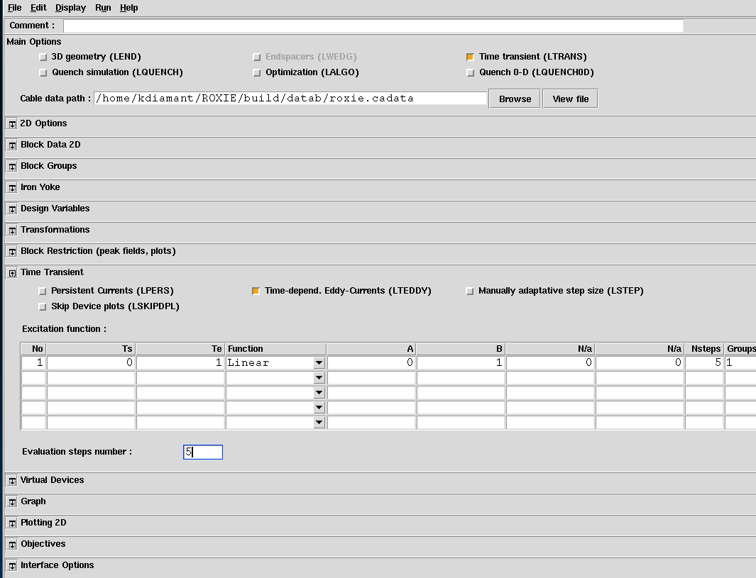
Chosen material and B-H data with corresponding conductivity are used. For this we should activate the LTRANS option for Time-Transient Analysis and LTEDDY for Time-Dependent Eddy-Currents.
Choosing our excitation function, Nsteps represent the number of "snapshots" for this excitation while Evaluation steps are the number of internal steps to refine the calculations.
As an example when we use a linear excitation of 1 second from A to B with Nstep=2 and Evaluation steps=5, ROXIE will produce 2 snapshots @0.5sec and @1sec.
From 0 to 0.5 seconds: This is the first segment of time between the two snapshots. ROXIE will perform 5 evaluation steps during this interval. Each evaluation step represents a finer time increment where the simulation updates the current field and calculates the induced eddy currents. These intermediate steps (such as 0.1 sec, 0.2 sec, etc.) are not outputted—they’re used internally to ensure the simulation progresses smoothly. Only the result at 0.5 seconds is stored and plotted.
From 0.5 to 1 second: Similarly, the second segment between 0.5 and 1 second will also use 5 evaluation steps. Again, these are internal steps that refine the calculation at intermediate time points, but only the result at 1 second is stored and plotted.
Note that, the more the evaluation steps the more expensive the computations are. All the internal step results can be retrieved with the ROXIE-API.
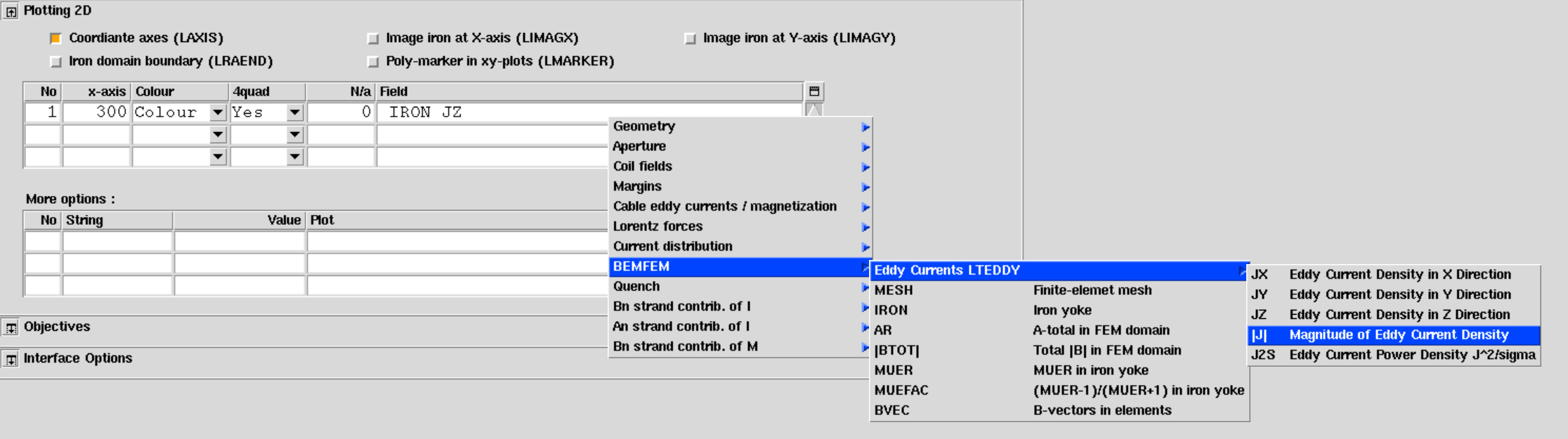
Under 2D plots the Eddy Current density J and Eddy Current Power desnity can also be visualized when running LTEDDY.