Examples of Interfaces
Interfaces for 2-D calculations
In this section we present interface files for the nested quadrupole-/dipole-model in Fig. 11.5.
Field-vector matrix (Map)
The "Field-Vector Matrix (Map)"-option in the "Interface Options"-widget produces an output file. In 2-D this happens only if a matrix-option (MATR, MATRC or MATRP from the "Aperture"-menu) is selected in the "Plotting Information 2-D"-widget.
  I   J         X          Y           BX          BY          |B|     DOMAIN
  1   1    -90.000000  -90.000000   -0.009448    0.043838    0.044844   B
  2   1    -80.526316  -90.000000   -0.016277    0.051280    0.053801   B
  3   1    -71.052632  -90.000000   -0.025893    0.058876    0.064319   B
  4   1    -61.578947  -90.000000   -0.038789    0.066333    0.076842   B
  5   1    -52.105263  -90.000000   -0.056004    0.073666    0.092538   B
  6   1    -42.631579  -90.000000   -0.080640    0.080640    0.114042   B
  7   1    -33.157895  -90.000000   -0.119580    0.082117    0.145060   B
  8   1    -23.684211  -90.000000   -0.172218    0.058646    0.181929   B
  9   1    -14.210526  -90.000000   -0.211407    0.001016    0.211409   B
 10   1     -4.736842  -90.000000   -0.219440   -0.072235    0.231023   B
 11   1      4.736842  -90.000000   -0.196080   -0.144229    0.243412   B
 12   1     14.210526  -90.000000   -0.144123   -0.203070    0.249015   B
 13   1     23.684211  -90.000000   -0.069422   -0.234215    0.244287   B
 14   1     33.157895  -90.000000    0.006643   -0.224513    0.224611   B
 15   1     42.631579  -90.000000    0.057199   -0.188974    0.197441   B
 16   1     52.105263  -90.000000    0.084098   -0.150712    0.172588   B
 17   1     61.578947  -90.000000    0.097002   -0.116668    0.151726   B
 18   1     71.052632  -90.000000    0.101551   -0.087620    0.134126   B
 19   1     80.526316  -90.000000    0.100762   -0.063251    0.118969   B
 20   1     90.000000  -90.000000    0.096463   -0.043178    0.105686   B
  1   2    -90.000000  -80.526316   -0.000995    0.049057    0.049067   B
  2   2    -80.526316  -80.526316   -0.007223    0.059286    0.059724   B
...  ...           ...        ...         ...         ...         ...  ...
The DOMAIN-column features 'F' or 'B', where 'F' means that the evaluation point is in a FEM domain and 'B' stands for a BEM domain.
The call of the "Field-Vector Matrix (Map)"-option together with a matrix-option (MATR, MATRC or MATRP from the "Aperture"-menu) prints the following lines to the .output-file:
     2-D MATRIX FIELD CALCULATION
     LONGEST VECTOR IN PLOT=    0.5439613      T
This output can be used to select a value for the "Vmax"-entry in the "Plotting Information 2-D"-table with the "More Plot Options"-option switched 'on'. This feature is used in BEM-FEM calculations when the evaluation of the field on BEM-FEM domain-boundaries yields unphysical singularities. The respective field vector is then calculated as a mean value of the surrounding field points. The output to the .matrf-file is adjusted in the same way.
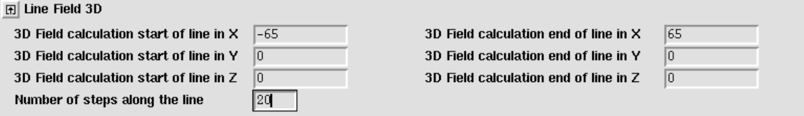
Field along a line (2-D, 3-D)
The "Field Along a Line (2-D, 3-D)"-option produces a postscript plot, compare Fig. 15.1 with the following input.
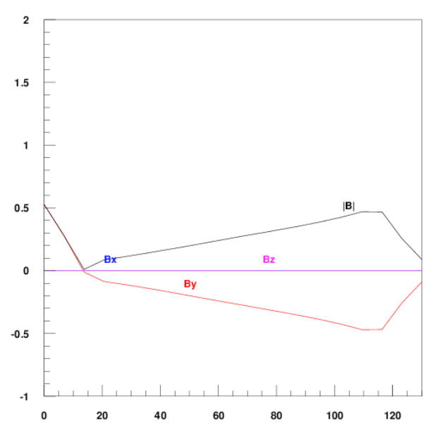
The line-field is also printed to the .output-file:
      CALL OF 3-D FIELD ALONG A LINE

  FIELD CALCULATION ALONG A LINE (SOURCE)

 I    X-POS   Y-POS   Z-POS   DIST      BX          BY         BZ        |B|
  1  -65.00    0.00    0.00    0.00  0.5767E-15  0.5270E+00  0.00E+00  0.53E+00
  2  -58.16    0.00    0.00    6.84  0.6543E-15  0.2775E+00  0.00E+00  0.28E+00
  3  -51.32    0.00    0.00   13.68  0.5068E-15 -0.1123E-01  0.00E+00  0.11E-01
  4  -44.47    0.00    0.00   20.53 -0.6157E-16 -0.8537E-01  0.00E+00  0.85E-01
  5  -37.63    0.00    0.00   27.37  0.2154E-16 -0.1097E+00  0.00E+00  0.11E+00
  6  -30.79    0.00    0.00   34.21 -0.1347E-15 -0.1351E+00  0.00E+00  0.14E+00
  7  -23.95    0.00    0.00   41.05  0.2429E-16 -0.1621E+00  0.00E+00  0.16E+00
  8  -17.11    0.00    0.00   47.89  0.5974E-16 -0.1900E+00  0.00E+00  0.19E+00
  9  -10.26    0.00    0.00   54.74 -0.8568E-16 -0.2183E+00  0.00E+00  0.22E+00
 10   -3.42    0.00    0.00   61.58 -0.9502E-16 -0.2467E+00  0.00E+00  0.25E+00
 11    3.42    0.00    0.00   68.42  0.1283E-16 -0.2749E+00  0.00E+00  0.27E+00
 12   10.26    0.00    0.00   75.26  0.4646E-16 -0.3029E+00  0.00E+00  0.30E+00
 13   17.11    0.00    0.00   82.11  0.2118E-16 -0.3311E+00  0.00E+00  0.33E+00
 14   23.95    0.00    0.00   88.95 -0.2125E-15 -0.3602E+00  0.00E+00  0.36E+00
 15   30.79    0.00    0.00   95.79  0.1845E-16 -0.3917E+00  0.00E+00  0.39E+00
 16   37.63    0.00    0.00  102.63  0.5219E-16 -0.4276E+00  0.00E+00  0.43E+00
 17   44.47    0.00    0.00  109.47 -0.1697E-15 -0.4692E+00  0.00E+00  0.47E+00
 18   51.32    0.00    0.00  116.32  0.1063E-15 -0.4675E+00  0.00E+00  0.47E+00
 19   58.16    0.00    0.00  123.16  0.6014E-16 -0.2577E+00  0.00E+00  0.26E+00
 20   65.00    0.00    0.00  130.00 -0.2660E-15 -0.8968E-01  0.00E+00  0.90E-01

      MAXIMUM OF THE FIELD COMPONENTS BX,BY:    6.5427821E-16   0.5269822
Coilmesh File
The "Ansys"-option creates a coilmesh.iron-file which contains one area-definition for each conductor in the cross-section.
kpcon1_1=[  0.070129,  0.001852];
kpcon1_2=[  0.070149,  0.000132];
kpcon1_3=[  0.085150,  0.000132];
kpcon1_4=[  0.085126,  0.002192];
lncon1_1=Line(kpcon1_1,kpcon1_2);
lncon1_2=Line(kpcon1_2,kpcon1_3);
lncon1_3=Line(kpcon1_3,kpcon1_4);
lncon1_4=Line(kpcon1_4,kpcon1_1);
arcon1=Area(lncon1_1,lncon1_2,lncon1_3,lncon1_4,BHiron7);
Lmesh(lncon1_1,1);
Lmesh(lncon1_4,8);
kpcon2_1=[  0.070061,  0.003811];
kpcon2_2=[  0.070119,  0.002092];
kpcon2_3=[  0.085117,  0.002432];
kpcon2_4=[  0.085046,  0.004491];
  ...
Autocad
The "Autocad"-option produces a filename.dxfxy-file which contains an autocad-model of the coil cross-section.
 0
SECTION
 2
ENTITIES
 0
POLYLINE
 8
25
66
   1
 10
0.0
 20
0.0
 30
0.0
 70
   1
 0
VERTEX
 8
25
10
  50.12915678993
 20
   1.84861619463
 30
0.0
 0
VERTEX
 8
25
...
MS Excel
The "MS Excel"-option creates a filename.excel file that has the geometrical information of the bare cables in the cross-section. A second table gives the coordinates of the corners of each cable block. The tables are comma-delimitted.
     CONDUCTOR POSITION IN THE CROSS-SECTION
     NO., COND., BLOCK , CORNER ,    X(mm) ,    Y(mm)
        , NO.  , NO.   , NO.    ,          ,
     1,    1,    1,    1,         50.1292,         1.8486
     2,    1,    1,    2,         50.1486,         0.1287
     3,    1,    1,    3,         65.1496,         0.1287
     4,    1,    1,    4,         65.1263,         2.1886
     5,    1,    1,    1,         50.1292,         1.8486
     6,    2,    1,    1,         50.0488,         3.8072
     7,    2,    1,    2,         50.1073,         2.0882
     8,    2,    1,    3,         65.1044,         2.4282
     9,    2,    1,    4,         65.0344,         4.4870
    10,    2,    1,    1,         50.0488,         3.8072
    11,    3,    1,    1,         49.8919,         5.7620
    12,    3,    1,    2,         49.9893,         4.0447
    13,    3,    1,    3,         64.9749,         4.7245
    14,    3,    1,    4,         64.8582,         6.7812
    15,    3,    1,    1,         49.8919,         5.7620
    16,    4,    1,    1,         49.6585,         7.7105
    17,    4,    1,    2,         49.7948,         5.9959

     BLOCK POSITION IN THE CROSS-SECTION
     NO., BLOCK , CORNER ,    X(mm) ,    Y(mm)
        , NO.   , NO.    ,          ,
     1,    1,    1,        63.3850,      25.0434
     2,    1,    2,        68.0000,       0.0119
     3,    1,    3,        83.3006,       0.0119
     4,    1,    4,        78.1010,      29.2325
     5,    1,    1,        63.3850,      25.0434
     6,    2,    1,        44.8894,      22.8527
     7,    2,    2,        50.0000,       0.0087
     8,    2,    3,        65.3010,       0.0087
   ...   ...   ...             ...           ...
2-D Field Map in Coil
The "2-D Field Map in Coil"-option creates a filename.map2-D-file. The file contains the magnetic induction in the position of every strand in the cross-section.
    UNSPECIFIED

&MAGNET
    NPOLE=  0, NBLOKS= 20,SCX=0.001,SCB=1.0,ORIGIN='ROXIE',VERSION=9.0,
    RIRON=  0.0000,BREF=  1.0000,XREF= 0.017000,/
 BL. COND. NO.  X-POS/MM  Y-POS/MM   BX/T      BY/T     AREA/MM**2 CURRENT FILL FAC.
  1   1    1    50.5506    1.4257   -0.0125   -0.4930   0.7206    27.78  0.3698
  1   1    2    50.5604    0.5611   -0.0018   -0.4932   0.7206    27.78  0.3698
  1   1    3    51.3839    1.4399   -0.0139   -0.4640   0.7285    27.78  0.3658
  1   1    4    51.3938    0.5658   -0.0017   -0.4642   0.7285    27.78  0.3658
  1   1    5    52.2171    1.4541   -0.0148   -0.4360   0.7363    27.78  0.3619
  1   1    6    52.2271    0.5705   -0.0020   -0.4362   0.7363    27.78  0.3619
  1   1    7    53.0503    1.4682   -0.0157   -0.4089   0.7442    27.78  0.3581
  1   1    8    53.0604    0.5752   -0.0024   -0.4091   0.7442    27.78  0.3581
  1   1    9    53.8835    1.4824   -0.0166   -0.3825   0.7521    27.78  0.3543
  1   1   10    53.8938    0.5799   -0.0028   -0.3827   0.7521    27.78  0.3543
... ...  ...        ...       ...       ...       ...      ...      ...     ...
2-D line currents
The "2-D Line Currents"-option creates a filename.fila2-D-file. The file contains information on the current-carrying areas in every discretized conductor (compare the N1-, N2-parameters in the "Block Data 2-D"-table), as well as on the position of each line current. The file therefore contains two tables:
  POSITIONS OF CURRENT AREAS  (2-D)
  NO. OF THE FIL.,   CURRENT
  X1 , X2 , X3 ,  X4
  Y1 , Y2,  Y3,   Y4
        1    50.00000
        70.138903   70.129156   71.628868   71.638806
         0.992162    1.852107    1.886105    1.009161
        2    50.00000
        70.148649   70.138903   71.638806   71.648745
         0.132217    0.992162    1.009161    0.132217
        3    50.00000
        71.638806   71.628868   73.128579   73.138710
         1.009161    1.886105    1.920102    1.026160
              ...         ...         ...         ...

  POSITIONS OF CURRENT FILAMENTS  (2-D)
  NO.,   CURRENT         X            Y
        1    50.00000   70.883933    1.434884
        2    50.00000   70.893776    0.566439
        3    50.00000   72.383741    1.460382
        4    50.00000   72.393776    0.574939
        5    50.00000   73.883548    1.485880
        6    50.00000   73.893776    0.583438
        7    50.00000   75.383355    1.511379
      ...         ...         ...         ...
Write multipoles for Post-Processing
The "Write Multipoles for Pp."-option creates a filename.txt-file. The file contains the normal- and skew harmonics at every time-step. Every data line yields the step number, the time, the current in block 1, the main field component, and the relative harmonics.
Steps Time Current BN bn(n=1-20) an(n=1-20)
           1     0.00000  1000.00000    -0.26080 10000.00000  2685.33092   /
-23.36314     0.00000    12.63201     2.89206     1.27216     0.00000     /
0.01525    -0.00316    -0.01057     0.00000    -0.00231    -0.00001     /
0.00018     0.00000     0.00001     0.00000     0.00000     0.00000     /
0.00000     0.00000     0.00000     0.00000     0.00000     0.00000     /
0.00000     0.00000     0.00000     0.00000     0.00000     0.00000     /
0.00000     0.00000     0.00000     0.00000     0.00000     0.00000     /
0.00000     0.00000
Interfaces for 3-D calculations
In this section we present output files that can be produced to exchange data on 3-D coil end design with other programs. As a model coil end we use the end of Fig. 11.5, compare Fig. 15.2
Field vector matrix (Map)
The "Field-Vector Matrix (Map)"-option produces a filename.matrf-file which contains the components of the magnetic induction in the respective positions in the matrix.
     I , J , KK              1             1             1
     X , Y , Z      -80.000000    -80.000000      0.000000
     BX, BY, BZ      -0.001952      0.026444      0.002581
     I , J , KK              1             1             2
     X , Y , Z      -80.000000    -80.000000      5.128205
     BX, BY, BZ      -0.002208      0.029795      0.002715
     I , J , KK              1             1             3
     X , Y , Z      -80.000000    -80.000000     10.256410
     BX, BY, BZ      -0.002440      0.033063      0.002858
     I , J , KK              1             1             4
     X , Y , Z      -80.000000    -80.000000     15.384615
     BX, BY, BZ      -0.002637      0.036180      0.003011
        ...                ...           ...           ...
Field along a line (2-D, 3-D)
The "Field Along a Line (2-D, 3-D)"-option works in the same way in 3-D- as in 2-D-calculations.
CNC machining fiels
The "CNC Machine Files"-option, together with the "Wedge/Endspacer"-option in the "Main Options" produces a filename.cnc file that can serve as an input for a CNC-machining process of endspacers.
     $$ WEDGE    1 INNER, POLYGON    1 P. FOLLOW   23

     $$     X (mm)    Y (mm)    Z (mm)
      p     52.423    38.935     0.000
      p     52.423    38.935     9.313
      p     52.423    38.935    18.628
      p     52.423    38.935    27.946
      p     52.423    38.935    37.268
      p     52.423    38.935    46.592
      p     52.423    38.935    55.912
      p     52.423    38.935    65.219
      p     52.358    39.022    74.527
      p     52.041    39.444    83.813
      p     51.444    40.219    93.075
      p     50.546    41.342   102.274
      p     49.309    42.810   111.384
      p     47.682    44.615   120.383
      p     45.601    46.740   129.208
      p     42.981    49.160   137.807
      p     39.712    51.837   146.108
      p     35.668    54.698   153.982
      p     30.687    57.640   161.276
      p     24.612    60.484   167.723
      p     17.318    62.962   172.945
      p      8.864    64.696   176.413
      p      0.000    65.300   177.589

     $$ WEDGE    1 INNER, POLYGON    2 P. FOLLOW   23

     $$     X (mm)    Y (mm)    Z (mm)
      p     50.862    37.830     0.000
      p     50.862    37.830     9.327
    ...        ...       ...       ...
With the "Strips from Darboux Vec."-option the "CNC Machine Files"-option also produces a filename.darbcnc-file from the differential-geometry based coil-end design. The output format differs slightly.
$$ WEDGE    1 INNER, POLYGON ON OUTER RADIUS    P. FOLLOW 23

$$   X(mm)   Y(mm)   Z(mm)
p    51.310  40.406   0.000
p    51.391  40.360  102.320
p    51.463  40.326  98.876
p    51.330  40.536  100.616
p    50.859  41.140  106.361
p    50.069  42.085  114.134
p    49.336  42.941  119.923
p    48.722  43.655  123.849
p    48.218  44.255  126.479
p    47.746  44.824  128.473
p    46.890  45.766  131.551
p    45.480  47.192  135.873
p    43.532  49.003  140.894
p    41.065  51.083  146.216
p    38.155  53.276  151.455
p    34.918  55.435  156.288
p    31.320  57.526  160.704
p    27.314  59.513  164.683
p    22.850  61.349  168.177
p    17.851  62.974  171.131
p    12.317  64.281  173.416
p     6.333  65.142  174.880
p     0.000  65.450  175.395

$$ WEDGE    1 INNER, POLYGON ON INNER RADIUS    P. FOLLOW 23

$$   X(mm)   Y(mm)   Z(mm)
p    38.794  31.544   0.000
p    38.725  31.628  114.786
...     ...     ...      ...
Opera interface
The "Opera 8/20-Node Bricks"-option yields filename.opera8- and filename.opera20-files. They contain input for Vector Field's OPERA program that describes the coil ends in 3-D.
     CONDUCTOR GEOMETRY PRINT OUT FOR VF-OPERA 3-D
     ********************************************

     COND
     DEFI BR8
     0.0 0.0 0.0 0.0
     0.0 0.0 0.0
     0.0 0.0 0.0
           50.129157       1.848616       0.000000
           50.148649       0.128727       0.000000
           65.149612       0.128727       0.000000
           65.126267       2.188594       0.000000
           50.129157       1.848616      29.333333
           50.148649       0.128727      29.333333
           65.149612       0.128727      29.333333
           65.126267       2.188594      29.333333
          104.238036 , 1 , 0.0
      0 1 1
     10.
     QUIT
     COND
     DEFI BR8
     0.0 0.0 0.0 0.0
     0.0 0.0 0.0
     0.0 0.0 0.0
           50.129157       1.848616      29.333333
           50.148649       0.128727      29.333333
                 ...            ...            ...
Autocad
In 3-D calculations, "Autocad"-option produces not only a filname.dxfxy-file that describes the coil cross-section in an Autocad-readable format, but also a filename.dxfyz-file that yields the geometrical data of a cut through the $yz$-plane of a coilend.
 0
SECTION
 2
ENTITIES
 0
POLYLINE
 8
25
66
   1
 10
0.0
 20
0.0
 30
0.0
 70
   1
 0
VERTEX
 8
25
10
 228.98697156054
...
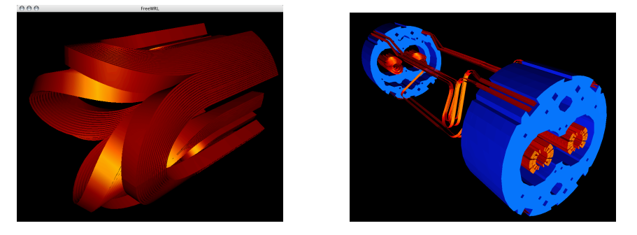
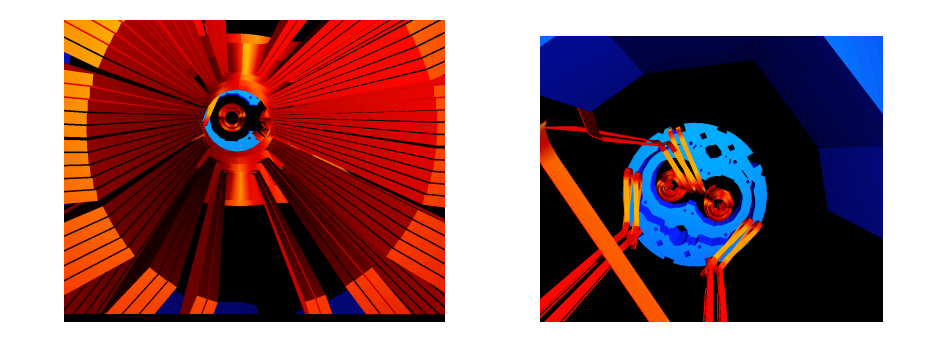
Virtual reality (3-D)
The "Virtual Reality (3-D)"-option produces a filename.wrl-file, which can be read in by any VRML-browser (sometimes called WRL-browser or VMRL-browser). A filename.wrl-file looks like this:
#VRML V2.0 utf8

Viewpoint {
  position 2 2 -20
  orientation 0 1 0 3.14
}

Group { children [ Transform {
    scale   0.0871   0.0871   0.0871
    children [ Shape {
      appearance Appearance {
        material Material {
           ambientIntensity  0.1
           diffuseColor      0.6 0 0
           specularColor     1 0.7 0
           shininess   0.02
      } }
      geometry IndexedFaceSet {
          coord Coordinate {
              point [
   68.1373    1.4818    0.0000,
   68.1489    0.1419    0.0000,
   83.1494    0.1419    0.0000,
   83.1356    1.7418    0.0000,
   68.1373    1.4818   36.6667,
       ...       ...       ...
The 3-D-model can be viewed in an interactive browser, compare Fig. 15.3.
3-D field map in coil
The "3-D Field Map in Coil"-option produces a filename.map3-D-file. The "3-D Peak Field Calc."-option in the "Global Information 3-D" must be switched 'on'. The file contains five tables which describe the position of the line currents (filaments), the field in $x$-, $y$-, and $z$-component, the the field in parallel-, perpendicular-, and longitudinal-component, the pressure on the conductors and the forces acting on the conductors.
     NFIL  NCUT  NCON      X         Y          Z
        1   1   1     68.5568      1.1522      0.0000
        1   2   1     68.5568      1.1522     36.6667
        1   3   1     68.5568      1.1522     73.3333
        1   4   1     68.5568      1.1522    110.0000
        1   5   1     68.5564      1.1565    116.3867
        1   6   1     68.5559      1.1699    122.7730
        1   7   1     68.5549      1.1924    129.1583
        1   8   1     68.5534      1.2242    135.5421
        1   9   1     68.5508      1.2653    141.9240
        1  10   1     68.5473      1.3374    148.3032
      ... ... ...         ...         ...         ...

     NFIL  NCUT  NCON      Bx        By       Bz        |B|
        1   1   1     -0.0136     -0.0929     -0.0001      0.0939
        1   2   1     -0.0164     -0.0986     -0.0002      0.0999
        1   3   1     -0.0173     -0.1122     -0.0003      0.1135
        1   4   1     -0.0152     -0.1300     -0.0010      0.1309
        1   5   1     -0.0127     -0.1353     -0.0005      0.1359
        1   6   1     -0.0091     -0.1376      0.0002      0.1379
        1   7   1     -0.0045     -0.1357      0.0012      0.1358
        1   8   1      0.0008     -0.1287      0.0024      0.1288
        1   9   1      0.0062     -0.1156      0.0040      0.1158
        1  10   1      0.0162     -0.0952      0.0080      0.0969
      ... ... ...         ...         ...         ...         ...

     NFIL  NCUT  NCON      B long.   B -|     B ||
        1   1   1     -0.0001      0.0939     -0.0144
        1   2   1     -0.0002      0.0999     -0.0173
        1   3   1     -0.0003      0.1135     -0.0182
        1   4   1     -0.0011      0.1309     -0.0163
        1   5   1     -0.0008      0.1359     -0.0153
        1   6   1     -0.0002      0.1379     -0.0162
        1   7   1      0.0005      0.1358     -0.0189
        1   8   1      0.0015      0.1287     -0.0226
        1   9   1      0.0026      0.1158     -0.0260
        1  10   1     -0.0005      0.0969     -0.0217
      ... ... ...         ...         ...         ...

     NCON  NCUT     P ||        P  -|        Px          Py          Pz
        1   1     -0.1018      0.0005     -0.1017     -0.0065      0.0000
        1   2     -0.1139      0.0006     -0.1138     -0.0080      0.0000
        1   3     -0.1057      0.0007     -0.1057     -0.0084      0.0000
        1   4     -0.0946      0.0006     -0.0945     -0.0075      0.0000
        1   5     -0.0905      0.0003     -0.0904     -0.0042      0.0000
        1   6     -0.0859     -0.0002     -0.0861      0.0013      0.0000
        1   7     -0.0808     -0.0008     -0.0821      0.0078     -0.0001
        1   8     -0.0747     -0.0014     -0.0786      0.0139     -0.0002
        1   9     -0.0672     -0.0018     -0.0753      0.0184     -0.0004
        1  10     -0.0566     -0.0023     -0.0708      0.0222     -0.0006
      ... ...         ...         ...         ...         ...         ...

     NCON  NCUT      Fr          Fphi       Fz
        1   1     -5.0024     -0.2598      0.0000
        1   2     -5.5976     -0.3265      0.0000
        1   3     -5.1962     -0.3507      0.0000
        1   4     -0.8139     -0.0543      0.0000
        1   5     -0.7810     -0.0255      0.0000
        1   6     -0.7528      0.0253     -0.0036
        1   7     -0.7308      0.0879     -0.0115
        1   8     -0.7153      0.1516     -0.0232
        1   9     -0.7044      0.2062     -0.0376
        1  10     -0.6915      0.2638     -0.0643
      ... ...         ...         ...         ...
3-D line currents
The "3-D Line Currents"-option creates a filename.fila3-D-file, which describes the positioning of line currents in 3-D coil models.
     NUMBER OF LINE CURRENTS *****
  12
  XS , YS , ZS
  XE , YE , ZE
  CURRENT
     12
         68.55680     1.15225     0.00000
         68.55680     1.15225    36.66667
         27.77778
     12
         68.55680     1.15225    36.66667
         68.55680     1.15225    73.33333
         27.77778
     12
         68.55680     1.15225    73.33333
         68.55680     1.15225   110.00000
         27.77778
     12
         68.55680     1.15225   110.00000
         68.55644     1.15654   116.38671
         27.77778
     12
         68.55644     1.15654   116.38671
         68.55587     1.16992   122.77296
         27.77778