Mathematical Optimization
Optimization
The ROXIE program was developed from the onset with mathematical optimization techniques in mind. This is reflected in the structure of the input files which allows, after the definition of the nominal geometry, to address any input data as a design variable of the optimization. The data structure also allows to define basically all computed data (and the design variables) as objectives for the optimization. The program structure is also reflected in the graphical user interface with its tables for design variables and objective function definition.
After many years of development many elements have found their way into the "Design Variables" which are mere transformations or input parameters for certain algorithms. In the same way post-processing options have found their way into to the "Objectives"-table. The user will quickly get used to the concept. It has, after all, allowed ROXIE to remain almost completely downward compatible to its previous versions as additional design variable or objectives do not alter the format of the .data-file.
Main options
| Option | Description |
|---|---|
| Optimization | Indicate that ROXIE should perform an optimization run. |
Design variables
The "Design Variables"-table has the following columns.
The table columns are called:
| Variable | Description |
|---|---|
| No | Row number. |
| Xl | Lower bound. |
| Xu | Upper bound. |
| Xs | Start value. |
| String | Design parameter/transformation parameter. |
| Act | The Blocks or Conductors the variables are applied |
During an optimization run, the design parameter is varied between Xl (lower) and Xu (upper), starting with Xs (start). To keep downward compatibility of the code, design variables can be "abused" for transformations or just as additional input parameters for subroutines and algorithms. In this case we set Xl=Xu=Xs. These data have to be grouped to the end of the design variable block. Design variables are parsed at every ROXIE run and the Xs values are always applied - even if no optimization has been chosen.
-
Transformations, i.e., Xl=Xu=Xs need to be grouped at the end of the table.
-
In the "Layer/Block/Cond./Strand" field we enter space-separated integer numbers. The following format is allowed:
1 4 7-9 10The "n-m"-entry is stored as "n (n+1) (n+2) ... (m-1) m". Note that per line no more than 20 layers, blocks, conductors or strands are stored.
Optimization:
Three options in this menu consider the neural-networks approximator for the EXTREM-optimization algorithm, see the "Extrem with ANN Approximator"-option above. The neural network is implemented in ROXIE but fragile.
| Variable | Description |
|---|---|
| STEPS | Number of steps for parametric study, compare the "Parametric Study"-option above. |
| NNEUR | Number of neurons for Radial Basis Function (default: 30) for Neural Network. |
| SSTAT | Threshold of S statistics (default: 1.3) for Neural Network. |
| NMLE | Threshold of NMLE (default: 0.0005) for Neural Network. |
Global information
Optimization algorithm
| Index | Option | Description |
|---|---|---|
| 0 | none | Do not optimize. |
| 1 | Extrem | Deterministic optimization algorithm. |
| 2 | Quasi-Newton DFP | Quasi-Newton- or Davidon-Fletcher-Powell algorithm. |
| 3 | Parametric Study | Variation of design variables within bounds without optimization. The number of steps is given in the STEPS-variable from the "Optimization"-menu of the "Design Variables". The results of a sequence of ROXIE runs are written to the .output-file. |
| 4 | Sensitivity Analysis | Determine sensitivity of the objectives with respect to tolerances in the design variables. |
| 5 | Levenberg-Marquard | Compromise between Newton's Method and the Method of Steepest Descent. |
| 6 | Lagrange Multiplier Estimation | Determination of the Lagrange-Multipliers in the optimality condition given by the Kuhn-Tucker equations. |
| 7 | Mutual Inductances in Non-Linear Circuits | Determination of the non-linear (differential) mutual inductances between layers. |
| 8 | Blocks Individually Powered | All blocks are powered successively, while the other blocks have zero current. Method to determine the impact of one block on the field quality. Today replaced by the Bn-options in the Bn Strand Contribution of I-menu of the "Plotting Information 2-D", see Section 6.1. |
| 9 | Random Multipole Error | Determine the mean-value and the standard-deviation of the multipole-components due to random changes of design parameters. Evaluate the Taguchi Function. |
| 10 | Genetic Algorithm | Use ROXIE's genetic algorithm for optimization. |
| 11 | Extrem with ANN Approximator | Use a neural network to accelerate the Extrem algorithm. This option is implemented but fragile. |
- The "Genetic Algorithm"-option does not allow to produce post-scripts during an optimization run. To take a look at the various families of designs, use the "Scan Through .scan-File"-option from the "Interface Options".
Objectives
The "Objectives"-table has the following columns.
| Variable | Description |
|---|---|
| Ne | Row number. |
| String | Right-click in a field of this column gives a list of objectives for optimization or plotting. |
| Nor | Specifies the objective, e.g., gives the order of the harmonic or the number of a strand/conductor. |
| Oper | Operand in the objective function or PLOT-operand. Right-click to get a list of operands. |
| Constr./Plot | If the operand in the objective function constitutes a constraint, then the value of the constraint is put here. With the PLOT-operand, the field gives the page number onto which the plot is to be drawn. |
| Weight | The weighting factor for the objective. Also used with the PLOT-operand. |
-
In order to plot graphs with the PLOT-operand, the "Postscript Plots"-option must be switched 'on'.
-
Whether or not the "Postscript Plots"-option is 'on', any optimization run produces a .post-file that contains two plots: The first plot shows the convergence behavior of the global objective function. The second plot gives the individual weighted objectives and their convergence.
The "Operand"-column yields a choice of operands.
| Operand | Description |
|---|---|
| MIN | Minimize the objective l, min(l). |
| MAX | Maximize the objective l, max(l). |
| MIN2 | Minimize the square of the objective l, $\mathrm{min}\left(l^2\right)$. |
| MAX2 | Maximize the square of the objective l, $\mathrm{max}\left(l^2\right)$. |
| MINI2 | Minimize the square of the inverse of the objective l, $\mathrm{min}\left(\frac{1}{l^2}\right)$. |
| MAXI2 | Maximize the square of the inverse of the objective l, $\mathrm{max}\left(\frac{1}{l^2}\right)$. |
| MINABS | Minimize the modulus of the objective l, $\mathrm{min}\left( |
| MAXABS | Maximize the modulus of the objective l, $\mathrm{max}\left( |
| < | 'Lower-than' constraint, $l<c$, with the upper bound $c$ given in the "Constraint/Plot"-column. |
| > | 'Greater-than' constraint, $l>c$, with the lower bound $c$ given in the "Constraint/Plot"-column. |
| =1 | 'Equals' constraint, $l{!\atop =}c$, with the constraint $c$ given in the "Constraint/Plot"-column. A linear (modulus) penalty is applied. |
| =2 | 'Equals' constraint, $l{!\atop =}c$, with the constraint $c$ given in the "Constraint/Plot"-column. A quadratic penalty is applied. |
| PLOT | Plot the objective during the optimization. The page on which to plot is given in the "Constraint/Plot"-column. Multiple plotting onto one graph is possible. The weights of the "Weight"-column are applied for the plotting. |
- As a general rule the quadratic operators MIN2, MAX2, =2 yield faster convergence if the start-set of design variables is far from the optimum solution. The 'modulus'-operators MINABS, MAXABS, =1 give better results for fine-tuning, when the start value is already a rather good design.
Global values:
| Variable | Description |
|---|---|
| NORM2X | L2-norm of the design variable vector. |
| NORM1X | L1-norm of the design variable vector. |
Interface options
| Option | Description |
|---|---|
| Scan Through .scan-File | The "Genetic Algorithm"-option in the "Optimization Algorithm"-variable of the "Global Information" produces a .scan-file with all design information of the different families of results. This option calls each design so it can be post-processed. |
| Cockpit-Software Output | Create a log-file to be read by the Tcl/Tk cockpit software for optimization, see Section The optimization cockpit |
The optimization cockpit
The cockpit software for optimization with ROXIE is started from the "Run"-menu. It can only be started with the "Optimization"-option in the "Main Options" and the "Cockpit Software output"-option in the "Interface Options" switched 'on'. An optimization run can then be started from the cockpit window and the design variables as well as the weighted objectives can be viewed online during optimization, see Fig. below. The main graph shows the convergence of the objective function. Moving the mouse cursor above the graph shows the individual function values obtained during optimization.
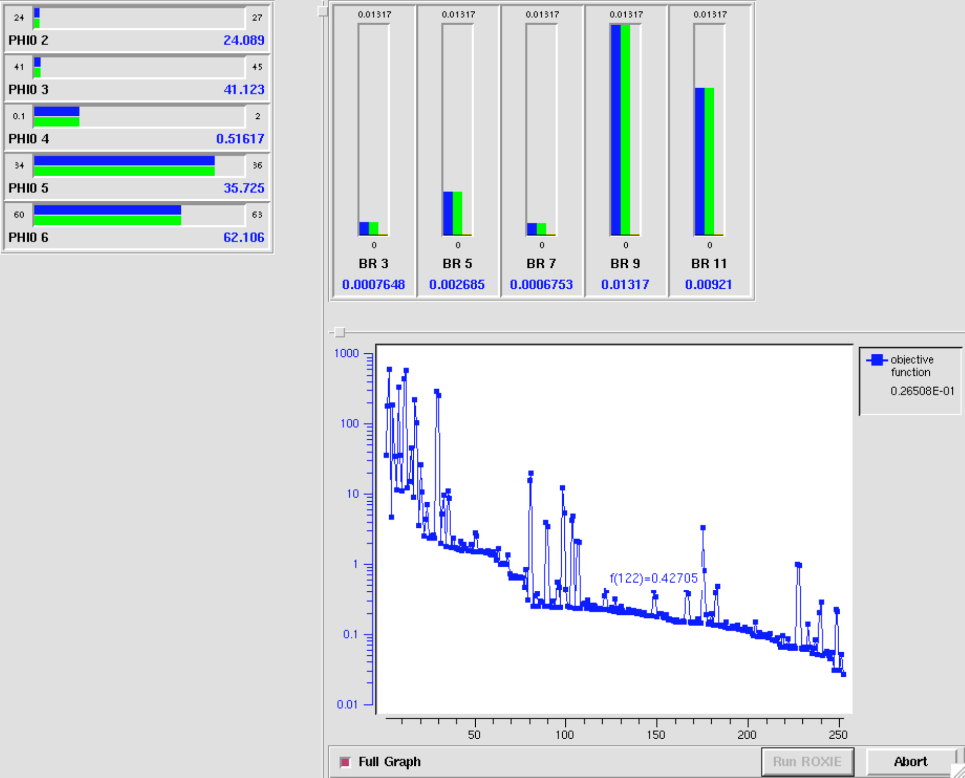
The cockpit window of ROXIE during an optimization run. Upper left: Design variables between lower and upper bounds. Upper right: Objectives between the absolute maximum and minimum values obtained during the optimization run. Lower right: Convergence of the objective function.
To use the cockpit window the following Tcl/Tk environment is recommended:
| Utility | Recommended Version |
|---|---|
| Tcl | 8.4.9 |
| Tk | 8.4.9 |
| BLT | 2.4 |
| BWidget | 1.7 |
All required software can be found on the internet, e.g., on http://www.sourceforge.net. Be aware that the BLT-toolkit does not work with the more recent version of Tcl/Tk 8.4.11!
Optimization with genetic algorithms
The genetic optimization routines in ROXIE are set up to handle bit-strings with about 60 bits. In order to use the algorithm, the optimization routines have to be enabled (LALGO=.true.) and the graphics output has to be disabled. Easy adaptation of pre-defined optimization parameters is foreseen. The genetic algorithm requires the number of bits for the discretization of each design variable. This parameter has to be entered in the column Xs of the design variable block instead of a start value, which is not needed in global optimization.
Genetic algorithms also allow for integer design variables. The only integer variables accessible to the ROXIE user are NUMCBL and those defined by the user in the .iron files. NUMCBL defines the number of conductors in each coil block. It is recommended to use discretization which correspond to the range of the integer variable. For a discretization by 2 bits for instance, $2^2$ different numbers of conductors can be generated. Choosing a bit string of length three, a coil block of 3, 4, 5, or 6 conductors can be chosen in the optimization. Therefore a range of 3 (Xa) to 6 (Xe) should be used in the setup. If the number of possible conductors is not dividable by the number of discretizations, the resulting non-integers are truncated in the optimization process.
Optimizing iron distributions
Currently the only design variable specified in the .iron file which can be addressed in the optimization is the material property. Instead of the BH-specifier (BH_air, and BHiron1 etc.) an integer variable may be used. The value 0 is equivalent to BH_air and all natural numbers are interpreted as the corresponding BHiron material. This definition allows for switching material regions from iron to air and for changes in the filling factor. For the latter case a list of material definitions has to be defined with appropriate filling factors in the roxie.bhdata file.
Definition of the objective function
In order to achieve good results the sensitivity of all design variables should be similar. The optimization interval should be set such that impossible or infeasible structures are avoided. Often, infeasible structures can be avoided by geometrical considerations.
Optimization parameters
The performance of the genetic algorithm can be influenced by an additional file named roxie.gadata. This file has to be created in the same directory as the .data file before starting the run. An example of a roxie.gadata file is given below:
60     ! Size of population
0.05   ! Rate of generation in percent
0.15   ! Rate of mutation in percent per iteration
6000   ! Number of iterations
Each number has to appear on a separate line. The comments on each line are optional. If the roxie.gadata file does not exist, default parameters are generated:
popsize = BIT_SIZE(child)
genrate = 0.05
mutrate = 0.0025*BIT_SIZE(child)
iterate = 100*BIT_SIZE(child)
Logging intermediate results
In order to avoid that results are lost in long genetic algorithm runs, a file roxie.gasafe is updated about every 2000 evaluations. The file has to be created before the first run, e.g., by typing 'touch roxie.gasafe'. In case of a stop, ROXIE can be re-started with the backup file. The optimization then continues from the last saved state. Each complete re-start of the genetic algorithm usually creates a new parameter set and therefore a new start population. The results of the optimization may therefore differ, since they depend on the original population. The niches found in each run, however, should be similar. A second local optimization stage may help in discriminating between distinct niches.
Post-processing
Evaluation of the optimization output can be done by reading the datasets from the scan-file. The scan-file contains the best 20 results of about every 2000th evaluation.