Examples of Numerical Field Calculation
Permanent magnets in 2-D
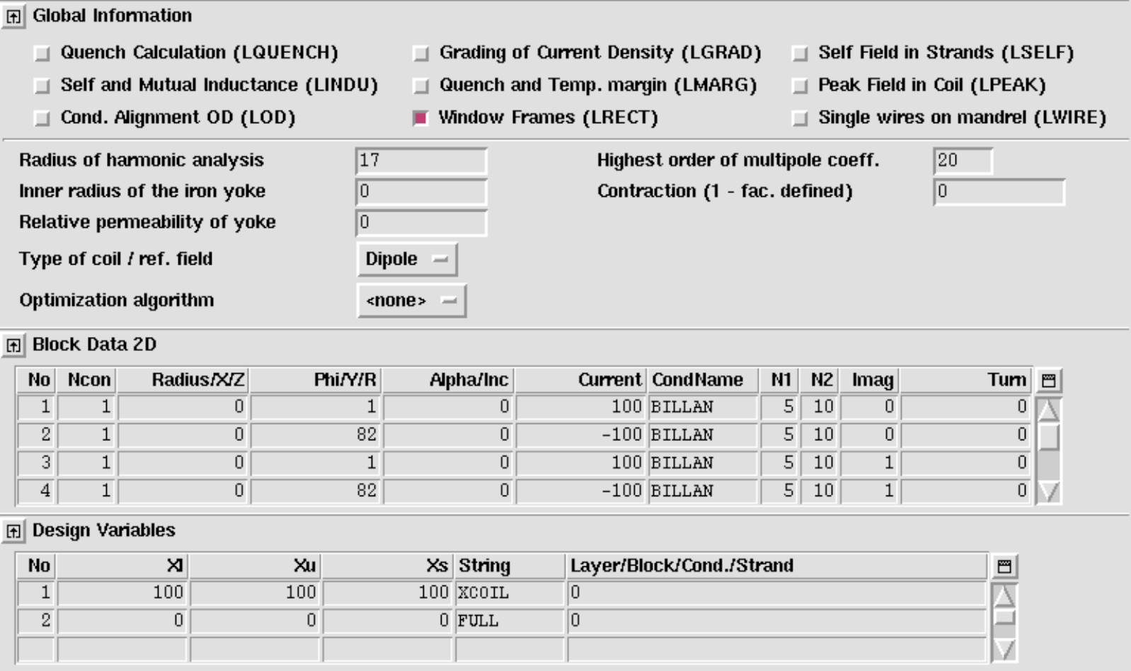
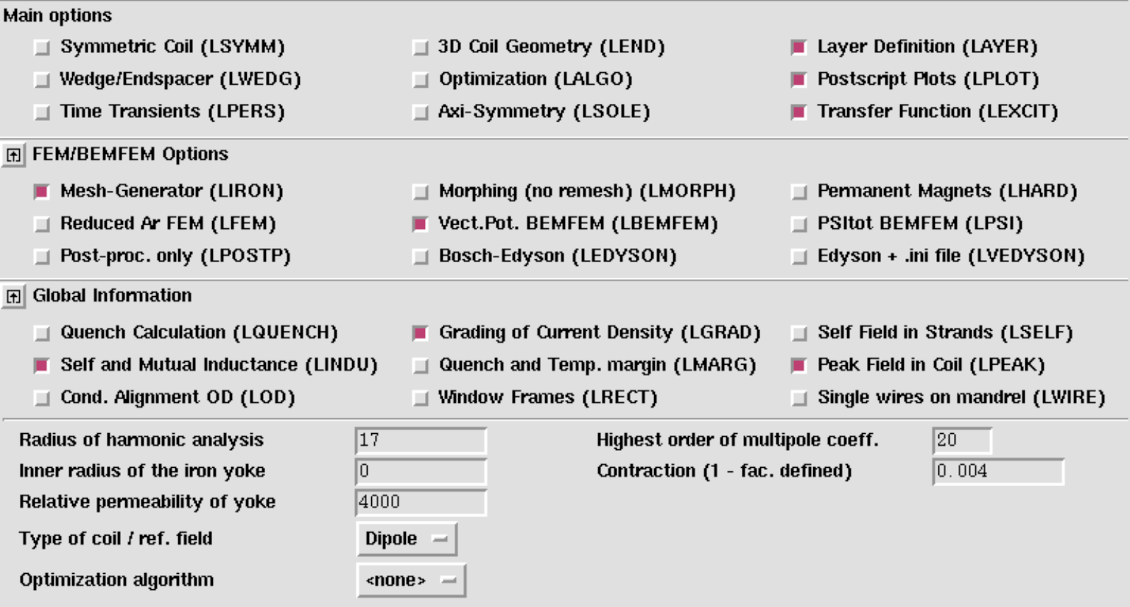
A 2-D calculation with permanent magnets is considerably more sophisticated than standard calculations with ferro-magnetic material. In a first step we create a standard model of the configuration with some kind of excitation coil. The following input illustrates this first step, compare Fig. 13.1. Note the shift of the radius of harmonic analysis by the XCOIL option. This is necessary as the origin for the finite element mesh generation was not chosen as the center of the aperture.
The .iron-file of this case is listed below, compare Fig. 13.1 (left).
-- IRON YOKE MODELLING FOR PERMANENET MAGNET CALCULATION
HyperMesh;

-- VARIABLES AND PARAMETERS
mm    = 0.001;
xpos1 = -52.0 * mm;     xpos2 = -2.0 * mm;      xpos3 = 150.0 * mm;       xpos4 = 2.0 * mm;
ypos1 = 0.0 * mm;       ypos2 = 32.0 * mm;      ypos3 = 80.0 * mm;

-- KEYPOINTS
kp1  = [xpos1,ypos1];       kp2  = [xpos2,ypos1];
kp3  = [xpos1,ypos2];       kp4  = [xpos2,ypos2];
kp5  = [xpos1,ypos3];       kp6  = [xpos2,ypos3];
kp7  = [xpos3,ypos3];       kp8  = [xpos3,ypos2];
kp9  = [xpos4,ypos3];       kp10 = [xpos4,ypos2];

-- LINES
ln1  = HyperLine(kp3,kp1,"Line",0.5);
ln2  = HyperLine(kp3,kp4,"Line",0.5);
ln3  = HyperLine(kp4,kp2,"Line",0.5);
ln4  = HyperLine(kp1,kp2,"Line",0.5);
ln5  = HyperLine(kp5,kp3,"Line",0.5);
ln6  = HyperLine(kp5,kp6,"Line",0.5);
ln7  = HyperLine(kp6,kp4,"Line",0.5);
ln8  = HyperLine(kp6,kp9,"Line",0.5);
ln9  = HyperLine(kp4,kp10,"Line",0.5);
ln10 = HyperLine(kp9,kp10,"Line",0.5);
ln11 = HyperLine(kp10,kp8,"Line",0.5);
ln12 = HyperLine(kp9,kp7,"Line",0.5);
ln13 = HyperLine(kp7,kp8,"Line",0.5);

-- AREAS
ar1 = Area(ln7,ln6,ln5,ln2,BHiron2);
ar2 = Area(ln13,ln12,ln10,ln11,BHiron2);
ar3 = Area(ln3,ln2,ln1,ln4,BHiron8);
ar4 = Area(ln10,ln8,ln7,ln9,BHiron9);

-- NUMBER OF ELEMENTS / LINE
Lmesh(ln1,6);

-- MIRRORING
Mirrorx;
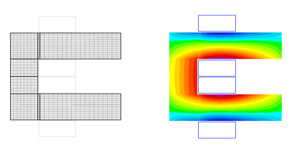
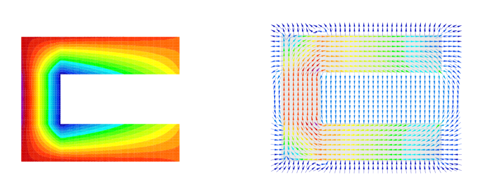
ar3 and its mirror image with
material BHiron8 are situated in the centre of
the arc; The areas ar4 and its image with
BHiron9 can be identified as the thin areas in
the branches. Right: Vector potential inside the C-magnet.
The materials BHiron8 and BHiron9 are defined in the
roxie.bhdata-file as permanent magnetic material. Their definition
reads
BHiron8
3 1.0
0.000    0.
0.9 7.0E+05
1.8 1.4E+06       permanent magnet material
BHiron9
3 1.0
0.000    0.
0.9 7.0E+05
1.8 1.4E+06       permanent magnet material
The definition of twice the same curve is necessary as two different
vector fields (directions) will later be assigned to the materials. We
can now identify the so-called collector-numbers of the areas with
materials BHiron8 and BHiron9 in the .hmo-file generated by the
HERMES pre-processor.
# HYPERMESH OUTPUT FOR EDYSON CREATED WITH MGEN2HMO; VERSION=1.3
BEG_COMP_DATA
       4
       1 BHiron9
       2 BHiron8
       3 BHiron2
       4 SuperCoils
END_COMP_DATA
BEG_NODL_DATA
    2473
       1  -0.00200000   0.08000000   0.00000000
       2  -0.00825000   0.08000000   0.00000000
       3  -0.01450000   0.08000000   0.00000000
       4  -0.02075000   0.08000000   0.00000000
          ...
BHiron9 has been assigned number 1 and BHiron8 has number 2. Finally
we can proceed to define two vector fields in a .VEFI-file, compare
Section 8.8.
    2    3
    1    1    0.9
    1    0    1   +2    0    0    0
  0.0  0.0  0.0  0.0  0.0  0.0
    2    2    0.9
    1    0    1   +1    0    2    0
  0.0  0.0  0.0  0.0  0.0  0.0
    2    0    1   -1    0    1    0
  0.0  0.0  0.0  0.0  0.0  0.0
This file defines 2 vector fields. The first one pointing in +y-direction and the second one pointing in +x-direction in the upper half plane and in -x-direction in the lower half plane.
In a final step we assign the vector fields to the respective areas (materials, collector numbers). The following input produces the output of Fig. Fig. 13.2. Note that all currents in the "Block Data 2-D"-table are now set to zero.
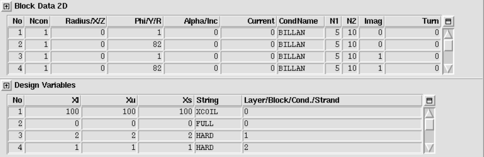
In Fig. Fig. 13.2 we used the NOCND-option in the "Plotting Information 2-D"-table to suppress the plotting of the current-void coil blocks.
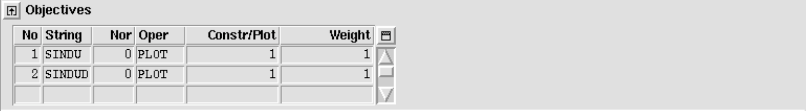
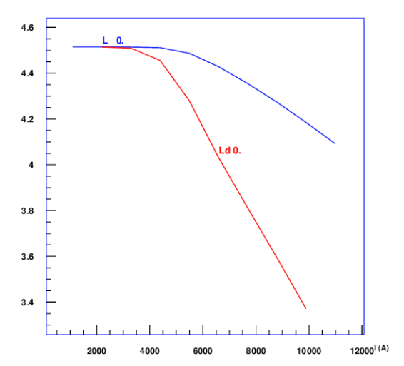
Differential inductance
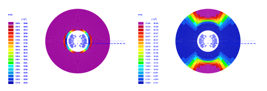
The calculation of a differential inductance of a magnetic circuit (compare is done during a transfer-function evaluation. If the induced voltage is measured during the ramping of the magnet, then it is the differential inductance that can be derived from these measurements. The following input automatically generates the output and plot shown in Fig. Fig. 13.3. Figure 13.4 shows the geometry with the iron yoke. On the yoke, the relative magnetic permeability is displayed at low field (left) and at high field (right).

Peak-field Calculation 3-D
To calculate peak fields in 3-D coil geometries, including the non-linear iron yoke magnetization, is a three-fold task:
-
In the first step the user finds the peak-field in the coil without iron yoke. To do this, we switch on the "3-D Peak Field Calc." option in the "Global Information 3-D", as well as the "3-D Field Map in Coil" in the "Interface options". Running the case without iron yields the peak field per block in the .output-file. The number of the conductor, which is exposed to the peak-field per block, is also given in the .output-file. From the .map3d-file we can then read the strand number where the peak-field occurs.
-
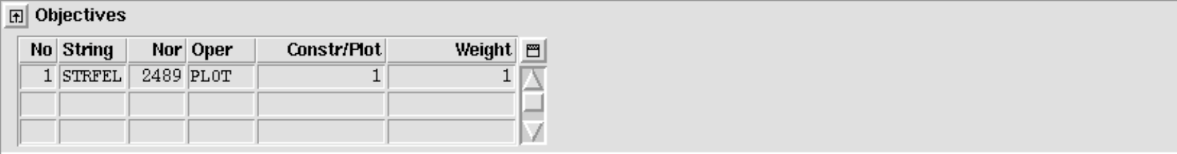
We now switch on the "Field along a line"-option in the "Interface Options" and supply dummy variables. Furthermore we choose the "STRFEL" ('strand field') option from the "Peak Fields"-menu in the "Objectives". For "Nor" we specify the peak-field strand number, for "Oper" the option "PLOT" and '1' for "Constr/Plot" and "Weight". The option "STRFEL" makes ROXIE calculate the field along a line, where the line is given by the strand geometry, from the straight section to the apex of the coil end. The output of the "Field along a line"-calculation is printed to the .output-file (see below) and a postscript plot is produced.
-
To make sure that the peak-field in the coil ends has not moved to another strand as a result of iron saturation, we have to repeat the calculation in the neighbouring strands. Which strands are adjacent to the specified strand can be found (relatively) easily from the first table in the .map3d-file and the preview window.
3-D peak-field printout in the .output-file:
     RESULTS OF THE 3D PEAK FIELD CALCULATION:

     BLOCK NUMBER ...............................           8

     B  ABSOLUTE IN TESLA .......................      5.3837
     B  TRANSVERSAL TO CURRENT DIRECTION (T) ....      5.3837
     B  IN DIRECTION OF CURRENT (T) .............      0.0027
     B  PARALLEL TO BROAD SIDE OF CABLE (T) .....     -5.1528
     B  PERPENDICULAR TO BROAD SIDE OF CABLE (T).      1.3407
     POSITION IN Z DIRECTION (NUMBER OF LAYER)...           3
     NUMBER OF CONDUCTOR WITH PEAKFIELD .........          70
     X KOORDINATE ...............................     14.4897
     Y KOORDINATE ...............................     50.0588
     Z KOORDINATE ...............................    314.4236
Corresponding .map3d-file entries.
          NFIL  NCUT  NCON      X         Y          Z
        1   1   1     62.1332     24.3131      0.0000
        1   2   1     62.1332     24.3131    314.8884
        1   3   1     62.1179     24.3614    333.4033
       ... ... ...       ...         ...         ...
     NFIL  NCUT  NCON      Bx        By       Bz        |B|
        1   1   1     -1.4857     -0.7931     -0.0090      1.6841
        1   2   1     -1.5525     -0.9637     -0.0062      1.8273
        1   3   1     -1.6063     -1.0023      0.0265      1.8935
       ... ... ...       ...         ...         ...         ...
     2488  19  70     -0.0326     -4.8824      0.6349      4.9236
     2488  20  70     -0.0110     -4.8769      0.6403      4.9188
     2488  21  70      0.0000      0.0000      0.0000      0.0000
     2489   1  70     -0.3210     -5.0882     -0.0190      5.0983
     2489   2  70     -0.3659     -5.3612      0.0973      5.3746
     2489   3  70     -0.3678     -5.3695      0.1322      5.3837
     2489   4  70     -0.3665     -5.3673      0.1582      5.3821
     2489   5  70     -0.3630     -5.3604      0.1863      5.3759
     2489   6  70     -0.3570     -5.3492      0.2163      5.3655
     2489   7  70     -0.3482     -5.3341      0.2482      5.3512
     2489   8  70     -0.3364     -5.3156      0.2814      5.3337
       ... ... ...       ...         ...         ...         ...
We see that the peak-field in block 8, conductor 70 is located in strand number 2489, position 3 (along the z-axis).
"Field along a line"-option with dummy variables:
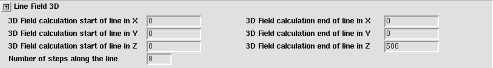
The strand-field option specifies the strand number 2489 for the "Field along a line" option.
The field-values along the strand number 2489 are printed to the .output-file.
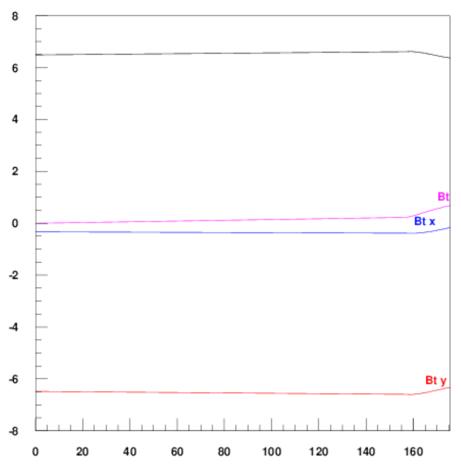
  FIELD CALCULATION ALONG A LINE (TOTAL)

   I    X-POS   Y-POS   Z-POS   DIST      BX          BY         BZ        |B|
    1   14.56   50.04  156.08    0.00 -0.3338E+00 -0.6476E+01 -0.7835E-03  0.6484E+01
    2   14.52   50.05  313.30  157.22 -0.3818E+00 -0.6595E+01  0.2236E+00  0.6610E+01
    3   14.43   50.08  315.00  158.92 -0.3836E+00 -0.6599E+01  0.2612E+00  0.6615E+01
    4   14.29   50.12  316.12  160.05 -0.3821E+00 -0.6594E+01  0.2890E+00  0.6612E+01
    5   14.09   50.18  317.25  161.20 -0.3784E+00 -0.6585E+01  0.3190E+00  0.6603E+01
    6   13.83   50.26  318.40  162.38 -0.3722E+00 -0.6570E+01  0.3511E+00  0.6590E+01
    7   13.49   50.36  319.57  163.60 -0.3630E+00 -0.6552E+01  0.3851E+00  0.6574E+01
    8   13.07   50.48  320.76  164.87 -0.3507E+00 -0.6531E+01  0.4206E+00  0.6554E+01
    9   12.56   50.62  321.94  166.17 -0.3351E+00 -0.6507E+01  0.4569E+00  0.6531E+01
   10   11.95   50.77  323.12  167.50 -0.3161E+00 -0.6480E+01  0.4936E+00  0.6507E+01
   11   11.23   50.94  324.28  168.87 -0.2940E+00 -0.6453E+01  0.5300E+00  0.6481E+01
   12   10.41   51.12  325.40  170.27 -0.2691E+00 -0.6425E+01  0.5656E+00  0.6455E+01
   13    9.49   51.30  326.46  171.69 -0.2418E+00 -0.6397E+01  0.5997E+00  0.6430E+01
   14    8.46   51.48  327.44  173.12 -0.2127E+00 -0.6371E+01  0.6317E+00  0.6406E+01
   15    7.35   51.65  328.32  174.55 -0.1821E+00 -0.6347E+01  0.6607E+00  0.6384E+01
   16    6.15   51.80  329.09  175.98 -0.1504E+00 -0.6325E+01  0.6862E+00  0.6364E+01
   17    4.87   51.93  329.72  177.42 -0.1178E+00 -0.6307E+01  0.7075E+00  0.6348E+01
   18    3.53   52.04  330.21  178.85 -0.8457E-01 -0.6293E+01  0.7241E+00  0.6336E+01
   19    2.15   52.11  330.55  180.27 -0.5119E-01 -0.6284E+01  0.7354E+00  0.6327E+01
   20    0.73   52.15  330.72  181.70 -0.1724E-01 -0.6279E+01  0.7412E+00  0.6323E+01

      MAXIMUM OF THE FIELD COMPONENTS BX,BY,BZ (ABS):    0.3835986
    6.599093       0.7412140
      MAXIMUM OF THE FIELD |B|:     6.615391
A postscript plot is produced:
Field Quality in a Bent Magnet
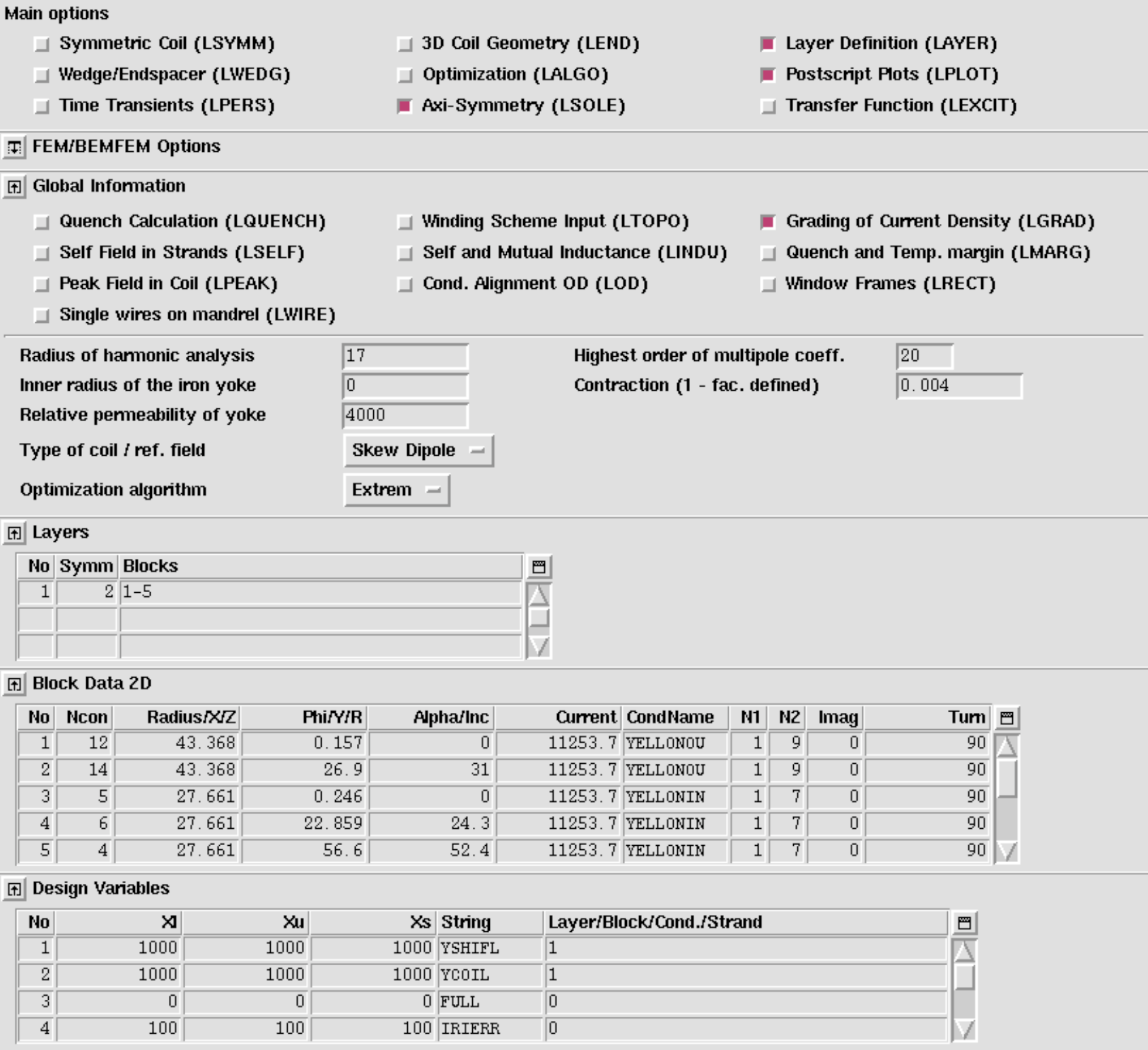
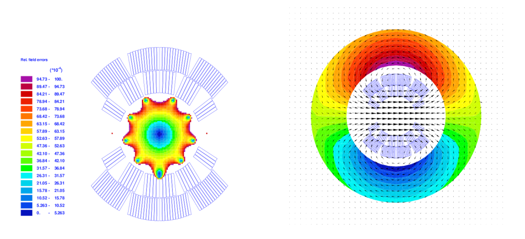
ROXIE can calculate the field quality in a long, bent magnet in a 2-D calculation. To this end we use the "Axi-Symmetry"-option in the "Main Options", which assumes that the x-axis is the axis of rotation.
If the magnet has a bending radius of 10 m, then we need to place the magnet 10 m above the x-axis. Moreover, we need to tilt the magnet by 90 degrees to make the bend axis coincide with the x-axis. We must create a full mesh of the iron yoke.
Peak-field and field-quality calculations will work. Time-transient calculations, however, are not implemented for the axi-symmetric case. They can be simulated for a "straight" cross-section.
The following input yields the plots in Fig. 13.5.