Examples of SC-Related Time-Transient Effects
The analytical models of SC magnetization
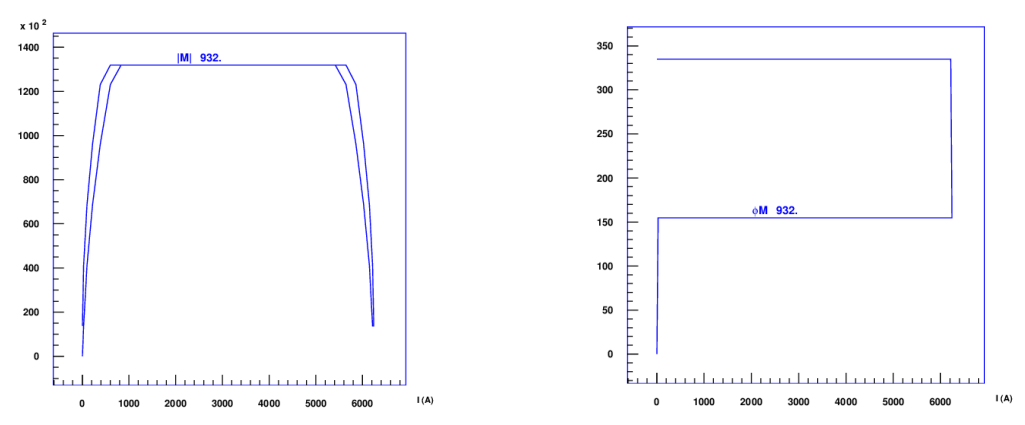
This section presents an example magnet and ramp cycle. The Persistent Current (PC) effects, the Interfilament Coupling Currents (IFCCs) and the Interstrand Coupling Currents (ISCCs) are simulated, their influence on field quality and loss-contribution are discussed. We use the following input in the "Time Transient Effects"-widget.
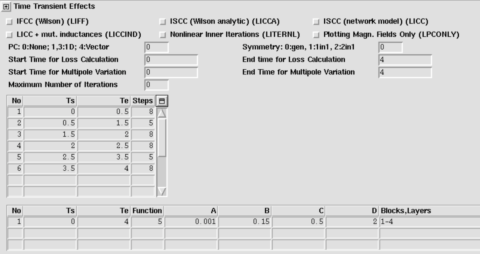
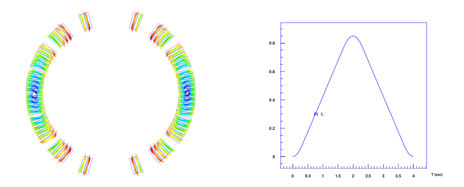
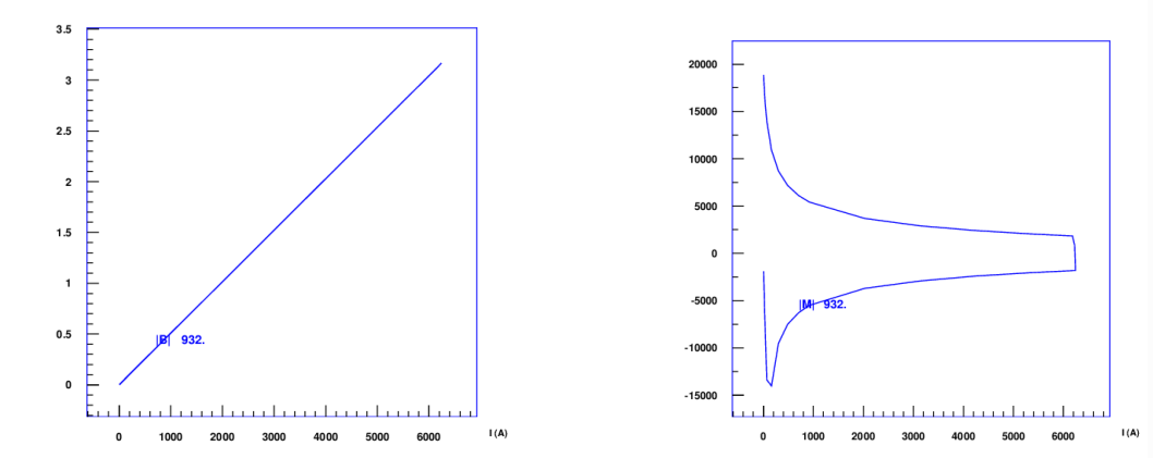
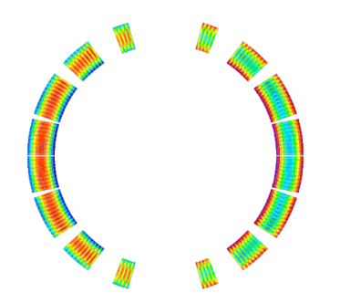
The excitation function thus defined is shown in Fig. 14.1 (right). The left plot shows the magnet cross-section and exciting magnetic field.
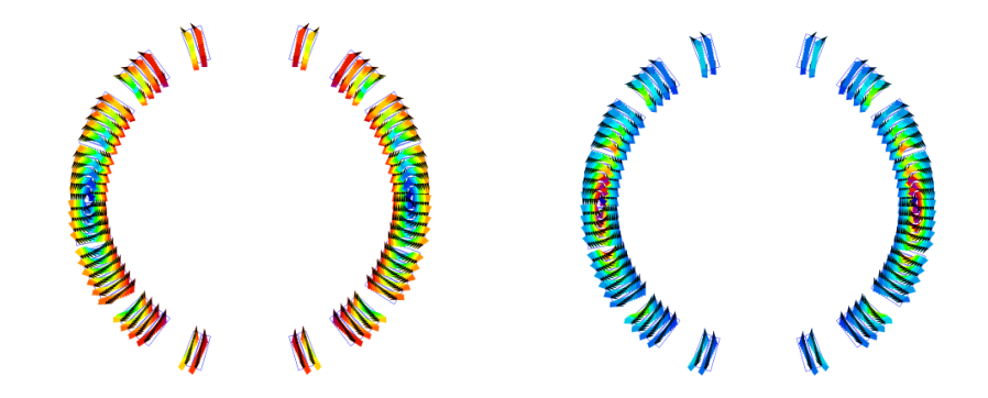

Persistent currents
The PC-magnetization of SC filaments is shown in Fig. 14.2. Figure 14.3 shows the excitation and magnetization curve of a single strand. Figure Fig. 14.4 yields the absolute and relative sextupole component of the field as a function of excitation current.
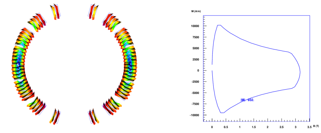
Interfilament coupling currents
The IFCC-magnetization of SC strands is shown in Fig. 14.5 (left). The right plot shows the magnetization curve of a single strand.
Interstrand coupling currents
The ISCC-magnetization of SC cables is shown in Fig. 14.6. Fig. 14.7 (left) shows the magnetization curve of a single strand in a cable. The right plot gives the angular information, including a jump by 180 degrees at the peak-excitation.
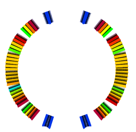
Note that analytical models of interstrand coupling currents can only give an estimate. Especially in terms of losses the implemented model tends to underestimate the real losses. This happens mostly when there are blocks with a field vertex, i.e., the magnetic field in a block shows in up on one side and down on the other, with zero field in the midle. In this case the cable-magnetization will underestimate the losses. The network model of Section 14.2 gives accurate results.
Network model of ISCCs
The same excitation as in the previous section is used to evaluate interstrand coupling currents from a network model which represents the cross-over- and adjacent resistances in a Rutherford-type cable. The coupling current pattern is plotted in Fig. 14.8.
Quench calculations
Quench simulation is, almost by definition, an ill-posed problem. The engineer can come up with an arbitrarily high number of design parameters, such as
-
for the the electrical network: power-supply, diode, dump resistor, ...,
-
for the electromagnetic problem: the geometry, material parameters of the yoke iron, cable parameters (adjacent- and cross-resistivities, time-constants...) ...,
-
for the protection instrumentation: detection thresholds, delays, quench heaters (heater power, discharge curve),
-
for the thermal problem: thermal conductivities, the cooling mechanism.
And at the same time there are only very few observables:
-
the current decay during a quench,
-
depending on the instrumentation of the quenching magnet, some voltage signals.
Moreover, many of the model parameters are notoriously difficult to determine.
The user must be aware that almost any quench simulation software, independent of its level of sophistication, will have enough parameters to fit a measured current decay curve. This does, however, not mean, that the quench behaviour of a magnet is understood and that the peak temperature is accurately predicted. On the contrary, for identical current decay curves, different models (with different sophistication) will yield differences in peak-voltages and peak temperatures of up to 50 percent.
We are nonetheless striving for more sophisticated quench modelling, because we wish to
-
understand the sensitivity of peak temperature and peak voltage to different model parameters, e.g.: Is an increase in RRR admissible? Can quench heaters be placed more efficiently? How do peak-voltages change if some quench heaters fail? By how much must the cooling increase to keep the peak temperature below specified values? What is the impact of increased/decreased adjacent and cross-over resistances? and many more questions.
-
avoid linearization where it is not applicable. The inductance of a magnet changes depending on the yoke saturation. For high-field magnets this effect is not negligible and can be modelled effectively.
-
have a qualitative understanding of a quenching magnet.
It is inevitable that the user studies the concepts of quench simulation in some detail. Moreover, a lot of information must be supplied to ROXIE to perform meaningful simulations. The theory of the present quench simulation algorithm in ROXIE is presented in the IEEE paper [@Schwerg:2007lr] by Nikolai Schwerg.
Winding Scheme
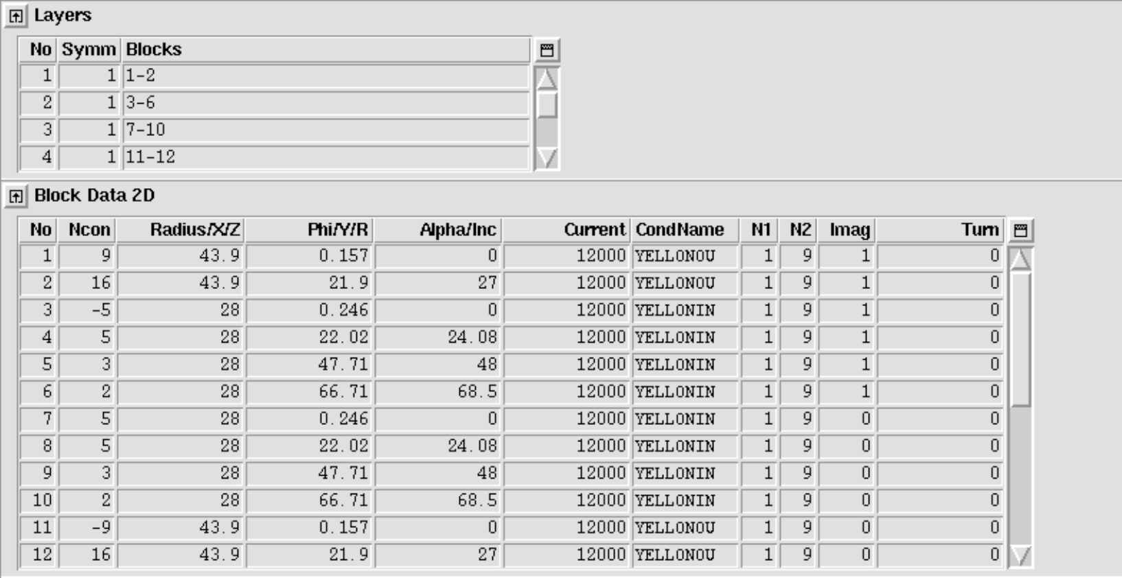
Until now the ROXIE program did not deal with coils as such, but with blocks and layers of conductors that were assigned excitation currents. For the calculation of internal voltages in coils during a quench, ROXIE must know the exact winding scheme, i.e. the succession of all conductors in the coil (or coil assembly). To provide this topological information, the user must use the "Layer"-option in the "Main Options". Only "Symm"-values 0 and 1 are admissible in the "Layers" widget.
The winding scheme can be previewed in the preview window if the "Winding Scheme Input"-option in the "Global Information" is 'on'. Then the conductor numbering according to the winding scheme is displayed after two successive clicks on the "1,2 ..."-button.
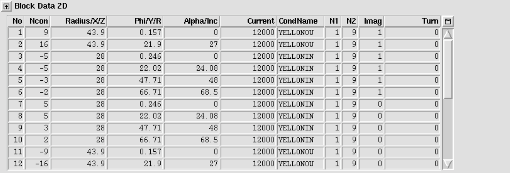
In order to obtain a correct winding scheme, the user can change the winding direction of individual layers: If the number of conductors "Ncon" in the "Block Data 2D" of at least one block in a layer has a negative sign, then the winding direction of the entire layer is inverted.
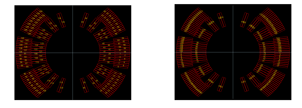
Don't forget that the winding-scheme numbering, which is displayed in the preview window if the "Winding Scheme Input"-option in the "Global Information" is 'on', is only used for the calculation of internal voltages. For all conductor-specific input in the design variables the conventional ROXIE numbering must be used, which can be previewed if the "Winding Scheme Input"-option is 'off'. The "Winding Scheme Input"-option only serves the purpose to toggle the conductor numbering in the preview window.
The following input produces conductor numbers with and without "Winding Scheme Input"-option that are displayed in Fig. 14.9.
Note that the following input in the "Block Data 2-D"-table produces an identical winding scheme as the above one.
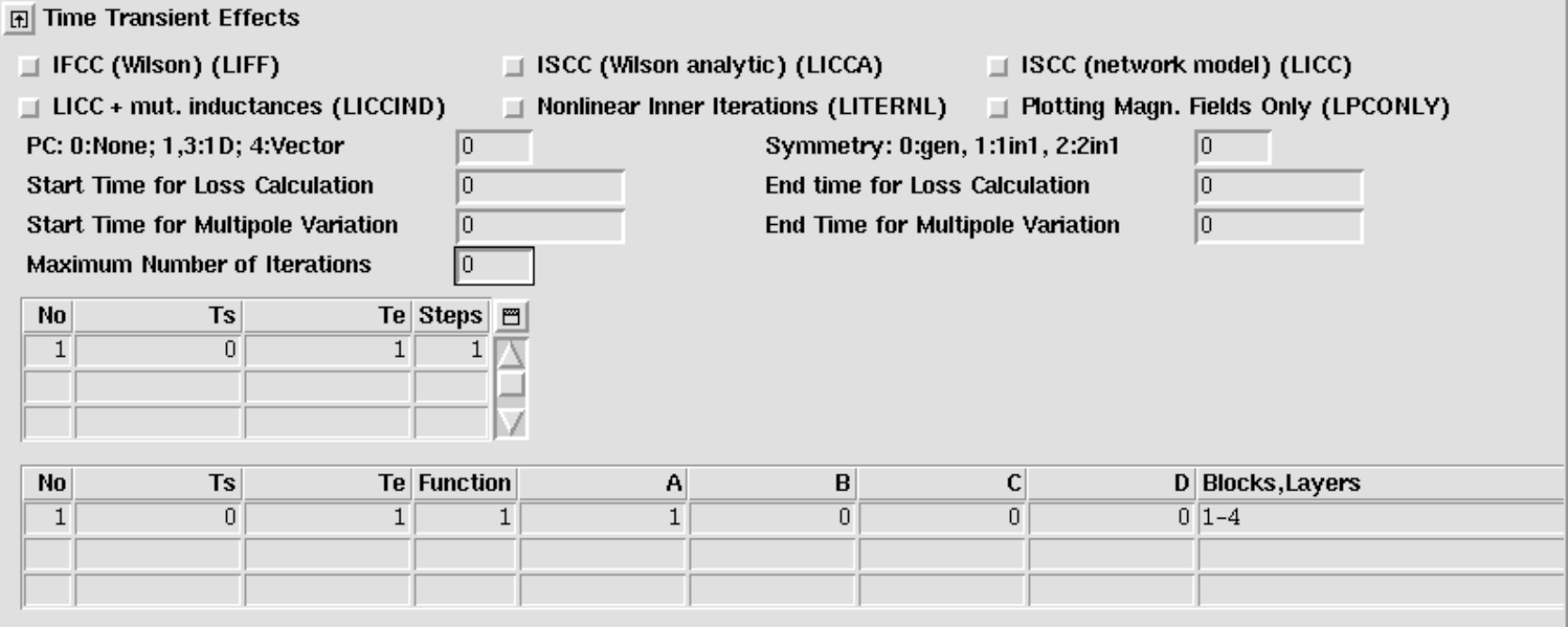
Transient Widget
Not all data in the transient widget is used for quench simulation. To take into account the quench-back effect, the user can choose between interfilament coupling current and/or interstrand coupling current models, see the respective sections in Chapter 9. Persistent-current losses are not considered for quench simulation at this stage of development.
We suggest only to use the "IFCC (Wilson)" option and the "ISCC (Wilson analytic)" option. All other options should be 'off', and the individual values all set to zero. The time-step table is not being used as the quench algorithm has an adaptive time-stepping algorithm.
At a later stage of development, ROXIE will be able to simulate a quench that occurs not at steady-state nominal conditions, but during an arbitrary excitation cycle. For the time being, however, the user has to supply a steady-state excitation of which the quench routine will only read the first time-step.
Basic quench
To do quench simulation, the following options must be set
-
"Quench Calculation" in "Global Information".
-
"Self and Mutual Inductance" in "Global Information".
-
"Quench and Temperature Margin" in "Global Information".
-
"Peak Field in Coil" in "Global Information".
-
"Time Transients" in "Main Options". For a description of the "Time Transients"-widget in the context of quench, see Section 14.3.
-
"Layer Definition" in "Main Options".
-
All conductors must be specified in the "Block spec." widget.
-
A winding scheme needs to be specified, see Section 14.3.
A minimum set of input parameters is given in the following screenshot:
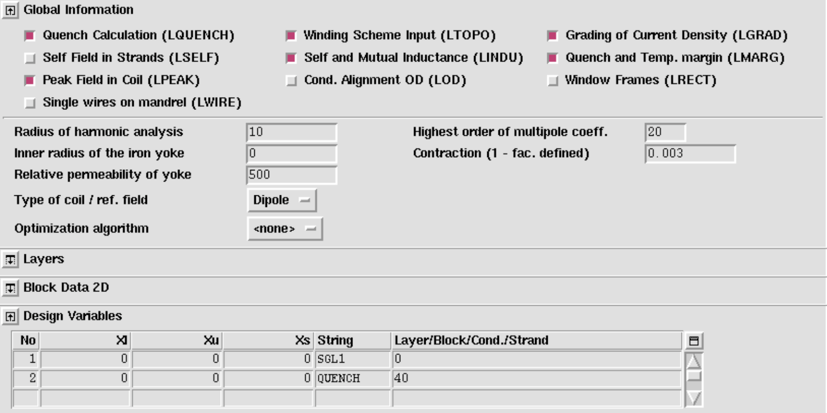
In this case, a quench originates in conductor 40 (compare left (!) picture in Fig. 14.9. There are no heaters, no delays, no diode threshold voltage, no dump resistors. The magnet is shortcircuited from t=0 s and dissipates its stored energy in the quenching zone. The RRR value is being read from the roxie.cadata-file. No quench back is considered. Azimuthal quench-propagation is not considered.
The full model
The full set of design variables is used in the following table
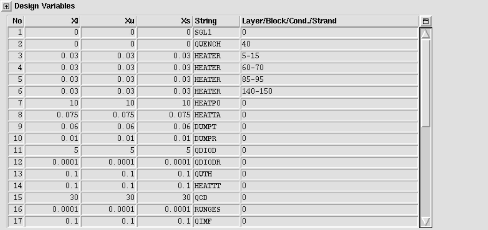
Furthermore a number of objective variables are implemented
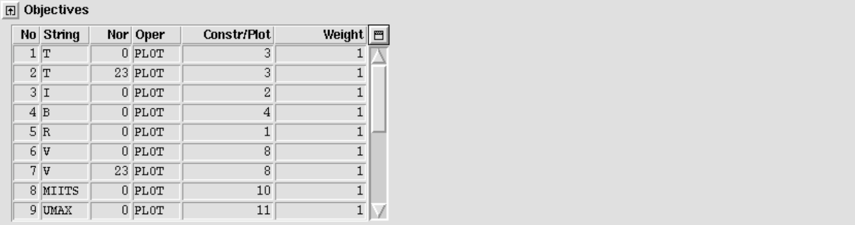
Note however that, if you use the objectives to produce figures, ROXIE is only capable to depict the first 200 timesteps (due to legacy). The parameters can be used without restriction in an optimization.
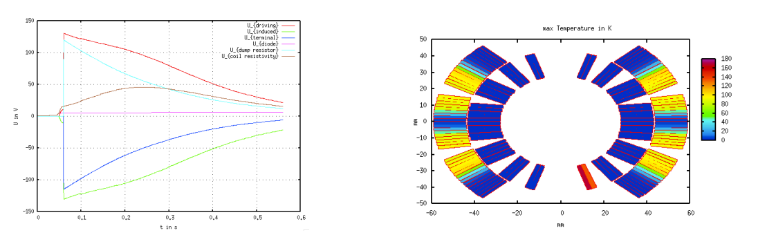
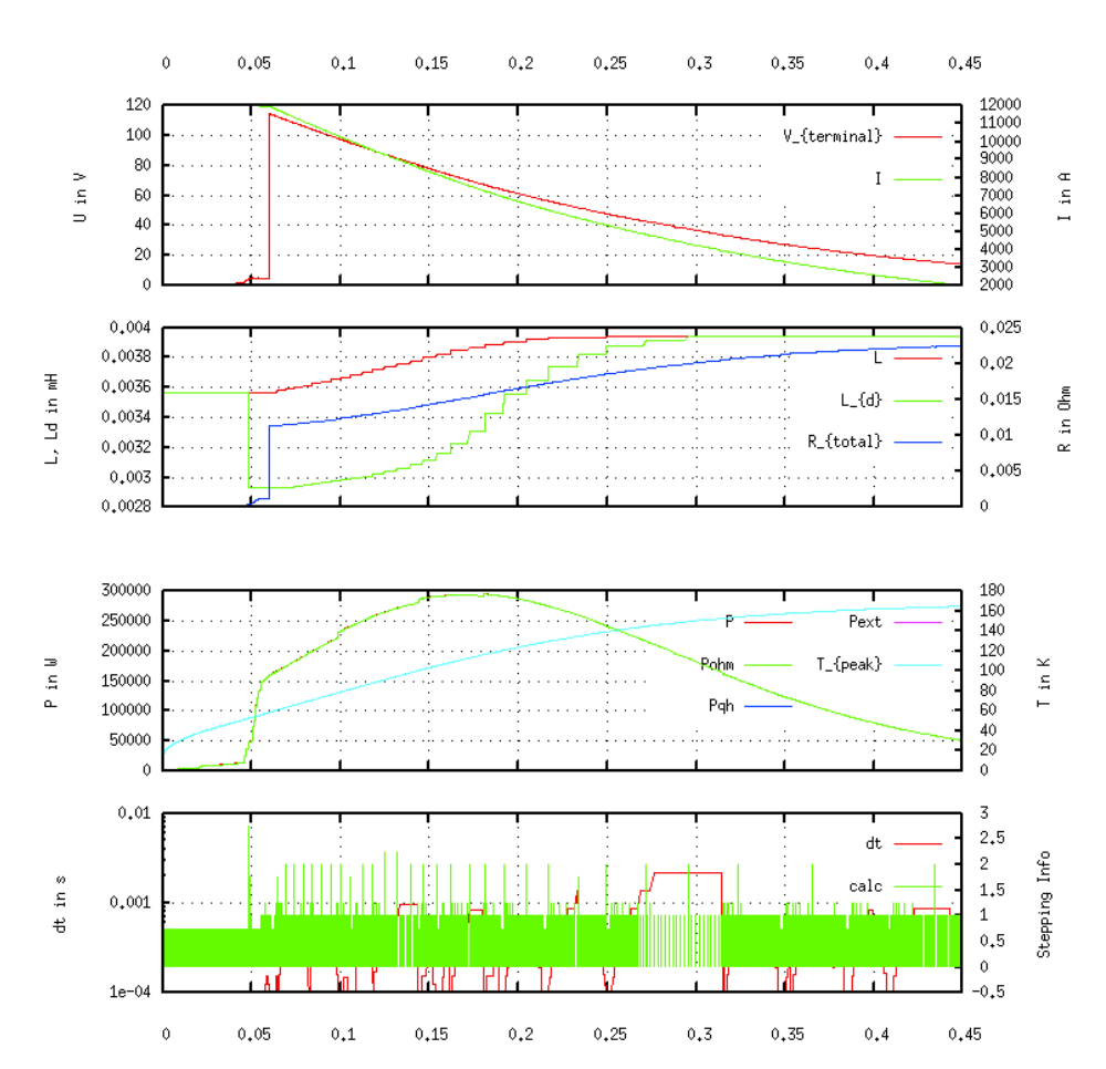
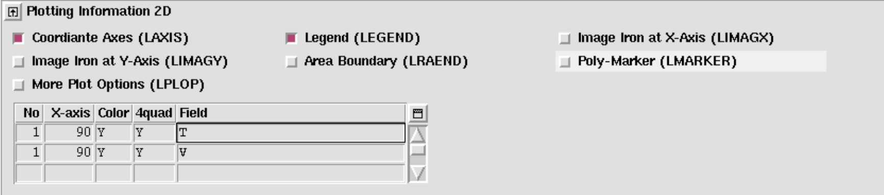
Cross-section plots of temperature and potential distribution can be produced
Extensive postprocessing is available via gnuplot files, e.g. the plots in Figs. 14.10 and Fig. 14.11, compare Section 9.3.