Mesh Generation

While the definition of the coil geometry is driven by a user's interface based on the Tcl/Tk script language (data stored in a file named filename.data), the input data for the mesh-generator has to be written into a file named filename.iron. To combine a coil with the appropriate iron yoke, the .data- and .iron-file must have the same name. The .iron-file can be opened from the Xroxie environment from the "Iron"-menu as soon as the "Mesh-Generator"-option is 'on' in the "FEM/BEMFEM Options".

In this section the rules and commands for the creation of the .iron-file are given together with an example. The HyperLine command supports design features for the creation of parametric meshes in magnet design.

General rules

• The lines are ended by a semicolon.

• To comment a line insert a '--' in front of it. Comments can also be added at the end of lines.

• Variables can be up to 100 characters long.

• The file has to start with the command "HyperMesh;". Omitting this command allows to be compatible to an older version of the mesh-generator.

Definition of parameters

• Scalar variables cannot start by kp,ln,ar, or BH

• All arithmetic operations plus the functions like Sin, Cos, Asin, Acos, Sqrt, and Tan are allowed in scalar expressions.

• Design variables are defined with the prefix dv and its value is given by ROXIE if they are defined as design variables in the .data file as well.

Definition of keypoints

• Keypoints are represented with variables starting with kp, e.g. kp1 or kpleft.

• Possible operation with keypoints: sum, scalar multiplication, subtraction.

• Keypoints are defined from the scalar expressions with the operators [xcoor, ycoor] for Cartesian coordinates and [radius @ angle] for polar coordinates.

• It is possible to access the coordinates of a keypoint as kp1.x for the x-componet and kp1.y for the y-component of keypoint kp1.

The HyperLine command

The HyperLine command was introduced to facilitate the input of complicated geometries. It is applied instead of the Line, Arc and Ellipse commands to define lines. The syntax is as follows:

ln1 = HyperLine(kp1,kp2,"string",arg1,arg2,arg3,arg4);

The "string" determines the type of the HyperLine. According to the chosen line type the arguments arg1-arg4 have different functions. Usually only some of them are user supplied, some of them can be defined optionally. The following sections summarise all different HyperLine types and explain the meanings of the parameters:

Curves & Arcs

Arc

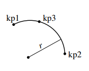
This is the keyword used for drawing a circular arc. arg1 is either the radius $r$ of the arc or the name of a third key-point (kp3). arg2 is optional and determines the linear contraction factor of the mesh (the default value is 0.5). For positive radii always the smaller arc segment is drawn, for
negative radii the bigger one.

ParabolicArc

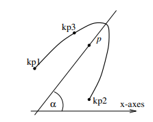
This string signifies that this line will be a parabolic arc. As first argument arg1 the parameter $p$ ($p$ defines the parabola by the equation $y^2=2px$) or a third key-point kp3 has to be supplied. arg2 is optional and determines the linear contraction factor of the mesh (the default value is 0.5). The third parameter is the angle $\alpha$. Its default value is 0.

EllipticArc

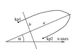
This keyword denotes an elliptic arc. The first and the second argument determine the two half axes $a$ and $b$ ($a$ and $b$ define the ellipse by $\frac{x^2}{a^2}+\frac{y^2}{b^2}=1$), the third argument arg3 (optional) is the linear contraction factor of the mesh (the default value is 0.5) and arg4 (optional) is the angle $\alpha$ (default is 0).

HyperbolicArc

A hyperbolic arc is drawn. The first and the second argument determine the two half axes $a$ and $b$, the third argument arg3 (optional) is the linear contraction factor of the mesh (the default value is 0.5) and arg4 (optional) is the angle $\alpha$ (default is 0).

Interpolation

This type is very similar to the old Ellipse command. The first argument arg1 has to be a third key-point. An interpolating function, equivalent to a finite-element shape function is drawn between the three key-points. The second argument is optional and denotes the linear contraction factor of the mesh (the default value is 0.5).

Line

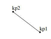
This command will connect kp1 and kp2 with a straight line. arg1 is optional and determines the linear contraction factor of the mesh (the default value is 0.5).

Element-macros of features used in magnet design

CornerIn & CornerOut

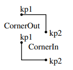
This line type creates a corner with both lines parallel to the y- and x-axes. This feature appears frequently in iron yokes of LHC magnets.

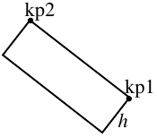
Bar

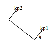
This line type creates three sides of a rectangle. The inclination and the orientation are determined by the sequence of the two key-points kp1 and kp2. The first argument arg1 (optional) is the height $h$ of the rectangle (negative values change the orientation). The default value of the height is half of the distance between the two key-points.

Notch

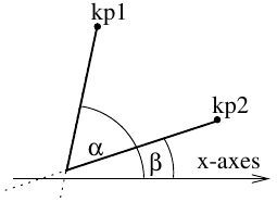
This line type creates a corner with two lines inclined by the angles α (arg1) and β (arg2). The default values are α = 0 and β = π/2.

Closed lines

These lines border an area themselves. However, the area has to be defined afterwards using the HyperArea command (see Section HyperArea command ).

Circle

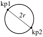
The "Circle" line type creates a circle with the two key-points kp1 and kp2 lying on a diameter.

Ellipse

This keyword will yield an ellipse with one half axes defined by the two key-points kp1 and kp2. The first argument (optional, default is $b=a$) either denotes the second half axes $b$ of the ellipse or is the name of a third key-point lying on the ellipse (kp3).

Rectangle

This line type will draw a closed rectangle defined by the two key-points kp1 and kp2 and the first parameter ($h=$ arg1). If no argument is supplied then a square is drawn.

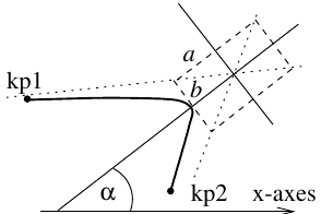
MillCut

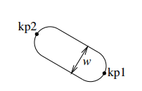
This keyword will create a closed line as shown on the sketch. The main symmetry axes is defined by two key-points kp1 and kp2. The first argument (optional, default is half of the distance between the two key-points) determines the width $w$ of the object.

The HyperArea command

The HyperArea command is an extension of the old Area command. In contrast to the old command which needed a closed polygon consisting of four lines only, HyperArea can define areas that are bordered by any number $N$ of lines. Of course the surrounding polygon has to be closed. If more than 2 lines are supplied the lines have to be ordered in a mathematically positive sense (anti clockwise). The exact grammar is as follows:

ar1 = HyperArea(ln1,ln2,...,ln N,material);

The names of the lines have to start with the two letters ln, but are free otherwise. For better understanding the lines have been enumerated in our example. The last argument of HyperArea is regarded as the material of the area. The name of the material can be BHiron1--BHiron9 referring to one of the nine $B$-$H$ curves given in the roxie.bhdata file or is simply BHair for a meshed air region (air region part of the FEM-domain) or BH_air for an air region without mesh (field computation via boundary elements).

The HyperHoleOf command

The HyperHoleOf command is necessary to define holes in areas. If for example area ar1 lies entirely in area ar2 (e.g. a hole in the iron yoke) the following line has to be included into the iron file after the definitions of both areas:

HyperHoleOf(ar1,ar2);

This signifies that ar1 is a hole of ar2.

The Lmesh command

The Lmesh command serves for defining the mesh density in the domain.

Lmesh(lnN,K);

Where lnN is the line number N and K is the number of element edges along that line.

Example of the ".iron" file for mesh generation

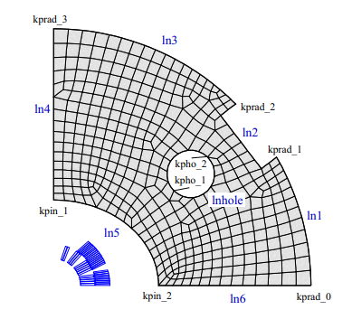
This is the example input file for the above case:

 HyperMesh;

 mm=0.001;                Pi=3.14159265;
 dv RADIUS=270;           radius=RADIUS*mm;
 dv RAD_HO=50;            rad_ho=RAD_HO*mm;
 dv ELL_A=110;            ell_a=ELL_A*mm;
 dv ELL_B=90;             ell_b=ELL_B*mm;

 kprad_0 = [radius @ 0];                            
 kprad_1 = radius*[Cos(Pi/6), Sin(Pi/6)];
 kprad_2 = [radius @ Pi/4];                         
 kprad_3 = [0 , radius];
 kpin_1  = [0 , ell_b];     
 kpin_2  = [ell_a , 0];
 kpho_1  =  kprad_1 - 2*[kprad_0.x-kprad_1.x,0];
 kpho_2  =  kpho_1 - [rad_ho/Sqrt(2.0), rad_ho/Sqrt(2.0)];

 ln1  = HyperLine(kprad_1,kprad_0,"Arc",radius,0.4);
 ln2  = HyperLine(kprad_1,kprad_2,"Bar",20*mm);
 ln3  = HyperLine(kprad_3,kprad_2,"Arc",radius,0.6);
 ln4  = HyperLine(kpin_1,kprad_3,"Line",0.4);
 ln5  = HyperLine(kpin_1,kpin_2,"EllipticArc",ell_a,ell_b);
 ln6  = HyperLine(kpin_2,kprad_0,"Line",0.4);
 lnhole = HyperLine(kpho_1,kpho_2,"Circle");

 aryoke = HyperArea(ln1,ln2,ln3,ln4,ln5,ln6,BHiron2);
 arhole = HyperArea(lnhole, BH_air);
 HyperHoleOf(arhole,aryoke);

 Lmesh(ln1,12);

Mesh extrusion for 3-D problems

To generate a 3-D mesh from a 2-D cross-section by extrusion, a file: \<filename>.extrude is needed. HERMES first generates a 2-D .hmo-file and then it runs HMO2HMO3-D, which produces a 3-D file by "extrusion" into $z$-direction.

The .extrude-file has one line for every extrusion of an area defined in the .iron-file.\

Variable	Type	Description
name	String	Area name starting with ar....
start	Double	$z$-position of start of extrusion.
end	Double	$z$-position of start of extrusion.
bias	Double	Biasing of mesh spacing towards start- or end-position of extrusion.
num	Integer	Number of elements in $z$-direction.
mat	String	Material name.

The material name entry is optional. If no name is given, the material of the .iron-file is chosen. The input must be uniform, i.e., all entries must have a material name or no entry has it.

In the example of Chapter 7{reference-type="ref" reference="chap:hermes"}, an .extrude-file looks like this

 aryoke -0.2 0.0 0.5 8 BHiron5
 aryoke 0.0 0.2 0.5 8 BHiron2

The above file produces a 3-D mesh of material BHiron5 from -20 cm to 0 cm in $z$-direction with 8 elements. Subsequently the 2-D mesh is extruded into BHiron2 from 0 cm to 20 cm. Note that, if the 2-D cross-section contains more than one area (holes must not be extruded!), then the extrusion interval in $z$ might be different for different areas. The author of the .extrude-file must ensure that the layers with element boundaries in $z$-direction match for all areas - even if the areas do not touch.

An extrude file for two areas, say aryoke1 and aryoke2 could look like this

aryoke1 0.0 0.4 0.5 3
aryoke2 0.0 0.4 0.5 3
aryoke2 0.4 0.5 0.5 1

Now aryoke1 and aryoke2 are extruded from 0.0 cm to 40.0 cm and aryoke2 continuous from 40.0 cm to 50.0 cm. In this examples the material is assigned to the areas that is specified in the 2-D .iron-file.